Drop test of a Phone

AIM:

To create a complete simulation file to perform a drop test from the given basic .k file consisting of only nodes and elements. To add the required keywords to create a solver deck to perform the drop test of cellphone.

OBJECTIVES:

• To create a solver deck to perform the drop test simulation.
• To select a unit system for the problem.
• To assign material properties for the cell phone and the rigid wall.
• To assign initial velocity for the cell phone.
• To create control keywords and desired output requests.
• To run the .K file and evaluate the results.

UNIT SYSTEM USED: G MM MS

MATERIAL PROPERTIES:

• Rigid wall: Here, the rigid wall is to be considered as the concrete road.

Density: 2300 kg/m³ = 2.300e^-3g/mm³

Youngs Modulus (E): 33GPa = 33e³ g/mm*ms²

Poissons Ratio: 0.21

• Cell Phone: Here, Steel material is used for the cell phone.

Density: 7850 kg/m³ = 7.850e^-3 g/mm³

Youngs Modulus (E): 200Gpa = 200e³ g/mm*ms²

Poissons Ratio: 0.25

Yield Strength: 210Mpa = 210 g/mm*ms²

PROCEDURE:

• Importing:
• FILE > OPEN > LS DYNA KEYWORD FILE > DROP_TEST_ONLYMESH.
• 
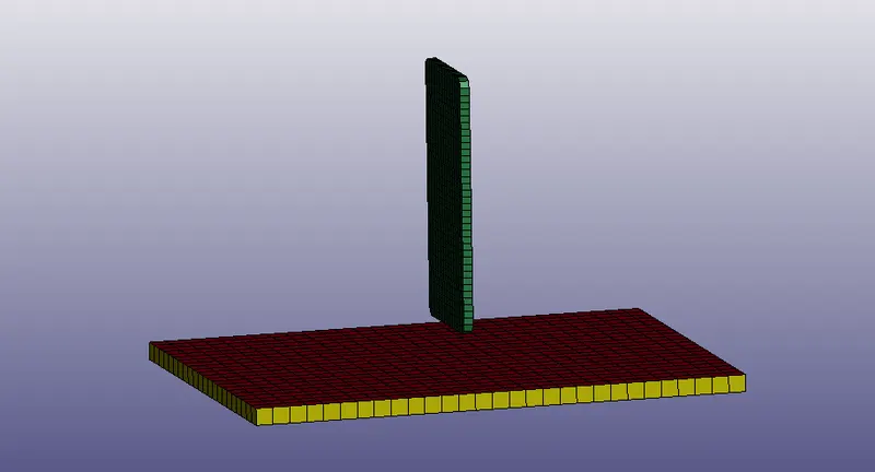
• Then, go to MODEL AND PART COMMAND > KEYWORD MANAGER.
• 
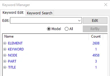
• We can check the keywords in the model.
• Part Check:
• Go to MODEL AND PART COMMAND > PART DATA.
• 
• We can see that the model consists 3 parts. Delete the shell part, as we are going to use the solid part for the rigid wall.
• Now, rename the parts as Cell_Phone and Rigid_wall.
• Now, in the part card we have to define section and material, so let’s create a Section and Material card.
• *Section:
• Go to MODEL AND PART COMMAND > KEYWORD MANAGER > ALL > SECTION > SOLID > TITLE = SOLID_SECTION > SECID = 1 > ACCEPT > DONE.
• 
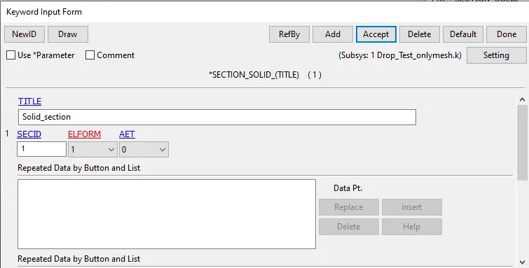
• This will create a solid section which can be defined for the parts.
• *Material:
• Go to MODEL AND PART COMMAND > KEYWORD MANAGER > ALL > MATERIAL > 24-PIECEWISE_LINEAR_PLASTICITY > TITLE = STEEL > MID = 1 > RO = 7.85E-3 > E = 2E5 > PR = 0.25 > SIGY = 210 > ACCEPT > DONE.
• 
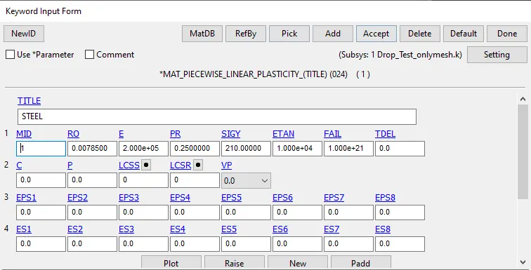
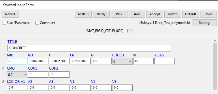
• Now, go to MODEL AND PART COMMAND > KEYWORD MANAGER > ALL > MATERIAL > 20-RIGID > TITLE = CONCRETE > MID = 2 > RO = 2.3E-3 > E = 33E3 > PR = 0.21 > ACCEPT > DONE.
• 
• Now, go to MODEL AND PART COMMAND > KEYWORD MANAGER > MODEL > PART > ASSIGN > SECTION AND MATERIAL.
• *Boundary_SPC:
• Now, we have to create Boundary condition for the Rigid_wall.
• Go to, MODEL AND PART COMMAND > CREATE ENTITY > CREATE > SET DATA > SET_NODE > PICK BY PART > RIGID_WALL > TITLE = RIGID_WALL > APPLY.
• 
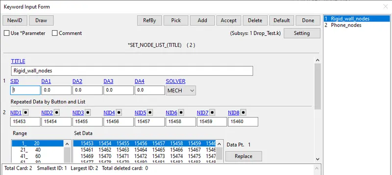
• This will create a Set node list for the rigid_wall.
• Again, MODEL AND PART COMMAND > CREATE ENTITY > CREATE > SET DATA > SET_NODE > PICK BY PART > CELL_PHONE > TITLE = CELL_PHONE > APPLY > DONE.
• This will create a Set node list for the cell_phone.
• Now, go to MODEL AND PART COMMAND > CREATE ENTITY > CREATE > BOUNDARY > SPC > CREATE > SET > NSID = 1 > ALL FIX > APPLY > DONE.
• This will define the rigid_wall as fixed boundary condition.
• *Initial_Velocity:
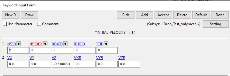
• Now, we have to define initial velocity for the Cell_phone.
• Go to, MODEL AND PART COMMAND > KEYWORD MANAGER > ALL > INITIAL > VELOCITY > NSID = 2 > VZ = -10 MM/MS > APLLY > DONE.
• 
• *Contact:
• Now, we have to define Contact for the Parts.
• Go to, MODEL AND PART COMMAND > KEYWORD MANAGER > CONTACT > AUTOMATIC_SURFACE_TO_SURFACE > CID =1 > TITLE = CELL_PHONE_TO_RIGID_WALL > SSTYP = 3 > MSTYP = 3 > SSID =3 > MSID = 4 > ACCEPT > DONE.
• 
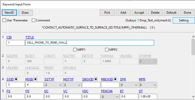
• This will define the contact as Slave for the Cell_Phone and Master for the Rigid_wall.
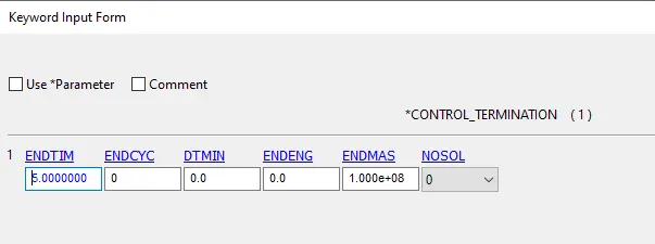
• *Control_Termination:
• Now, we have to define Control_Termination card for the simulation time.
• Go to, MODEL AND PART COMMAND > KEYWORD MANAGER > CONTROL > TERMINATION > ENDTIM = 5 MS > ACCEPT > DONE.
• 
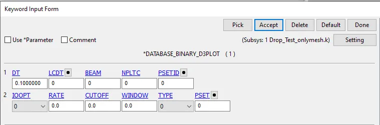
• *Database_Binary_D3plot:
• Go to, MODEL AND PART COMMAND > KEYWORD MANAGER > DATABASE > BINARY D3PLOT > DT = 0.1 > ACCEPT > DONE.
• 
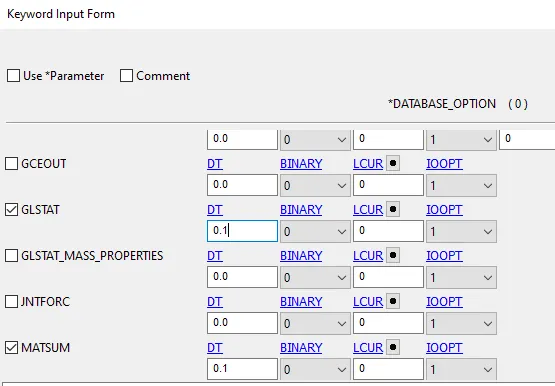
• *Database_ASCII:
• And finally we have to define the output results.
• Go to, MODEL AND PART COMMAND > KEYWORD MANAGER > DATABASE > ASCII > GLSTAT > DT = 0.1 MS > MATSUM > DT = 0.1 > ACCEPT > DONE.
• 
• Model check:
• The final step is to perform Model check.
• Go to, MODEL AND PART COMMAND > MODEL CHECK > DONE.
• 
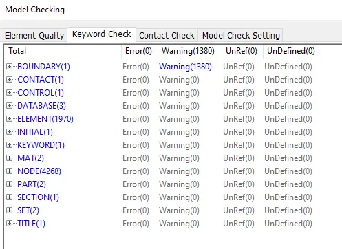
• As we can see, there are no errors in the model, hence we can proceed to simulation.
• LS_Run:
• Now, open LS RUN > OPEN THE FILE > RUN.
• 
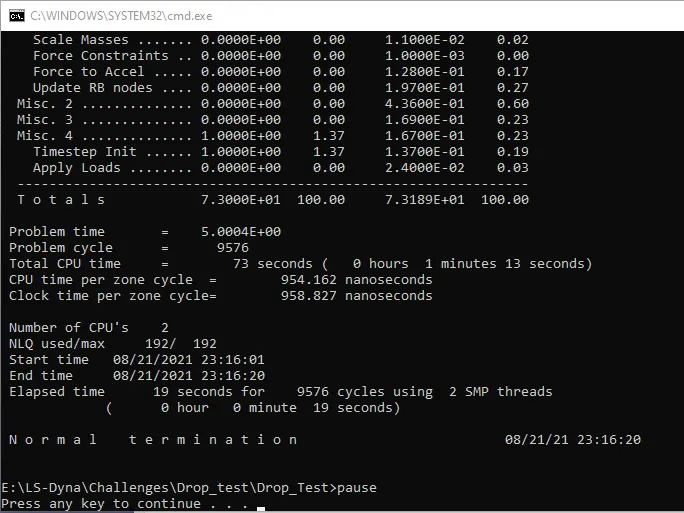
• The solver will solver the model and check for the Normal Termination message at the end of the solver screen.
• Post-Processing:
• Open LS Pre-Post.
• FILE > OPEN > LS DYNA BINARY PLOT.
• Go to, POST > FRINGE COMPONENT > STRESS > VON MISSES > DONE.
• 
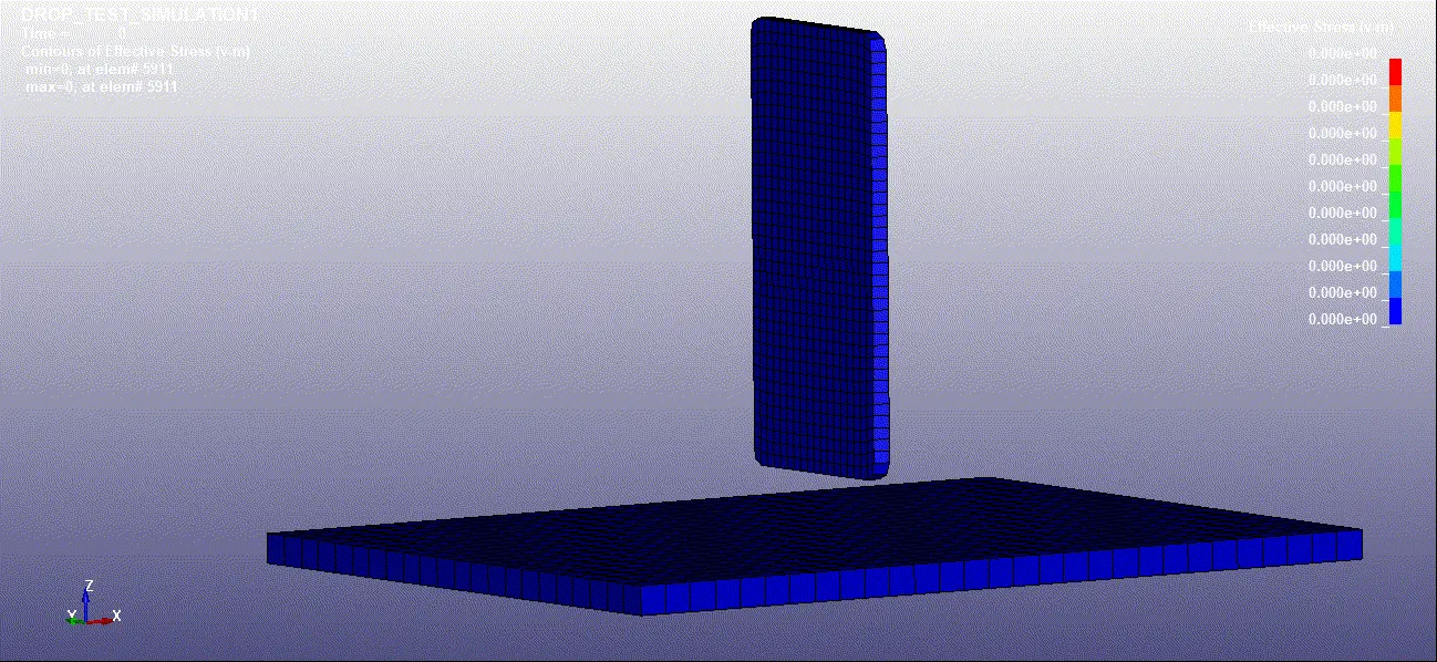
• To plot the Energy graphs go to, POST > ASCII > LOAD FILE > GLSTAT > SELECT ENERGIES > PLOT > DONE.
• 
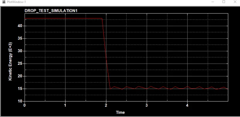
• As we can see that near 2 ms the cell phone impacts with the rigid concrete wall, the kinetic energy reduces as it is converted into internal energy.
• 
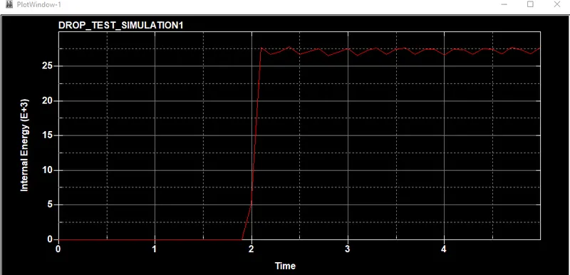
• The internal energy rises as the cell phone makes contact with the rigid wall.
• 
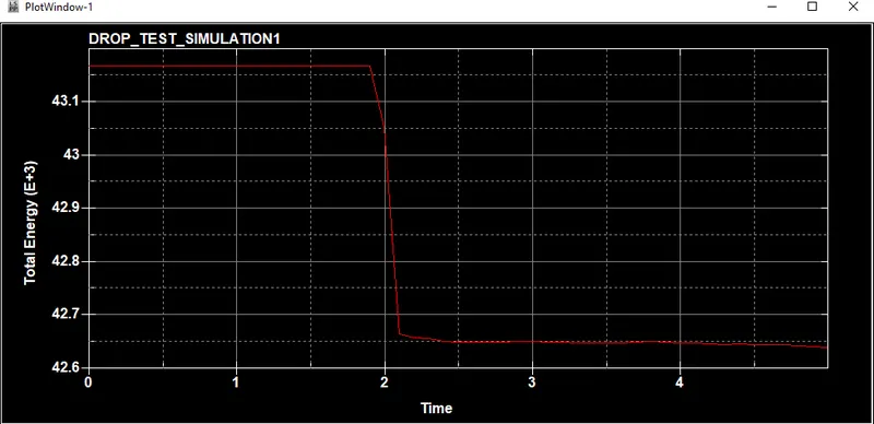
• This will plot the total energy graph for the model.

LEARNING OUTCOMES:

• To import the Keyword file.
• To check the model for parts data and keyword manager.
• To assign keywords for the model.
• To define section and material properties for the parts.
• To define set nodes.
• To define boundary conditions.
• To define initial velocity.
• To use Model check for checking the keyword manager.
• To define the output results.

CONCLUSION:

By performing this project we conclude that, the complete model setup was done and the model was simulated for drop test of cell phone.