MATLAB Program to Calculate and Plot Drag Force Against a Cyclist. (Matlab/Challenge-Week1)

Objectives

- To calculate Drag force and Coefficient of Drag for different velocities of the cyclist.

- To plot Velocity vs Drag Force Graph.

- To plot Drag Coefficient vs Drag Force Graph.

Theory -

Drag Force -

Drag Force is the resistance force experienced by a body by the fluid, whenever a body moves in a fluid medium (generally Air and Water). Drag force is expressed as the

following equation -

`D = 1/2 * Cd* rho*A*v^2`

Where, D = Drag Force

Cd = Coefficient of Drag

`rho` = Density of the medium

A = Reference Area (Usually Frontal Area of the Body )

v = Velocity of the moving body (or velocity of air for the stationary body)

Coefficient of Drag -

Coefficient of drag or Drag Coefficient (Cd) is a dimensionless no. which is most generally used for representing Drag on a body, as it contains all of the complex dependencies

of shape, inclination, and flow conditions on the body. It can be simplified from the Drag Force Equation as shown below -

`Cd = D/(1/2 * rho*A*v^2)`

It is also defined as the ratio of Drag Force to the force produced by the dynamic pressure times the area.

Represented as -

`Cd = D/(qA)`

Where, q = Dynamic pressure = `1/2 * rho*v^2`

Shape has a very large effect on the amount of drag produced. For the Same Frontal Area different shapes have different coefficient of drag.

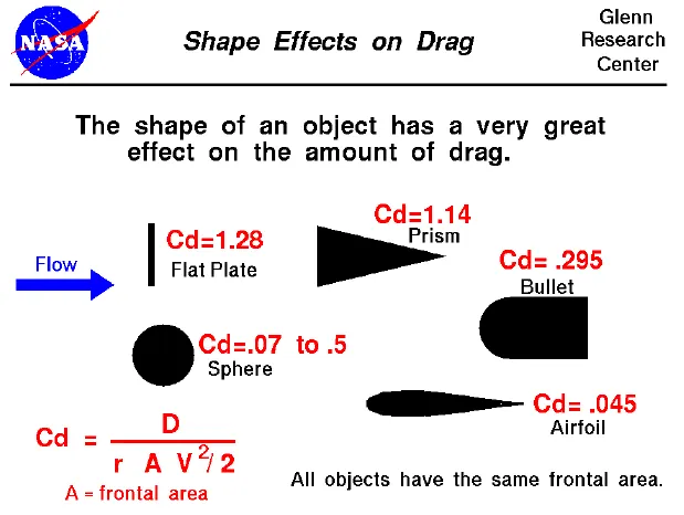
(Source: https://www.grc.nasa.gov/WWW/K-12/VirtualAero/BottleRocket/airplane/shaped3.html)

This happens mostly due to the factor of boundary layer separation. In shapes, in which boundary layer separation takes place early across the object's length(or chord length),

results in larger wake hence, leads to have higher Cd value in fact of having same frontal area.

Program -

- Drag force is to be calculated by using the above Equation.

Considering,

Frontal Area of Bicycle, A = 1 `m^2`

Density of air, `rho =1.225` kg/`m^3`

- For Plotting Velocity vs Drag Force Graph

We considered,

Drag Coefficient, Cd = 0.8 (Usually Cd of bicycle ranges between 0.6 - 1.1)

Velocity Range, v = 1 to 50 m/s

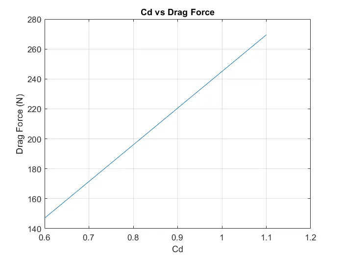
- For Plotting Cd vs Drag Force Graph

We know that for the same frontal area the drag coefficients differ for different shapes. In Bicycle, Cyclists have different seating positions, which changes the overall shape.

Following are some cyclists positions,

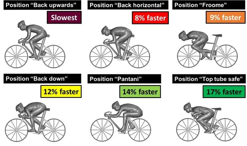
(Source: https://www.roadbikereview.com/threads/study-reveals-most-aero-position-on-bike.381203/)

Therefore, considering,

Drag Coefficient Range, Cd = 0.6 to 1.1 (Usually Cd of bicycle ranges between 0.6 - 1.1)

Constant Velocity, v = 20 m/s

Following is the Program -

%                 Program for Calculating the Drag Force of a Body(eg. here Bicycle)

clear all
close all
clc

A = 1;          % Frontal Area of the body here, 1 m.sq.
rho = 1.225;    % Density of the air, kg/m^3

%------------------ For Velocity vs Drag Force -------------------

cd = 0.8;                % coefficient of drag
v = linspace(1,50,50);   % Velocity range for the bicycle from 1m/s to 50m/s

D = 0.5*rho*A*(v.^2)*cd;  % Drag Force Equation, D-Drag Force

figure(1)
    plot(v,D);
    title('Velocity vs Drag Force');
    xlabel('Velocity (m/s)');     ylabel('Drag Force (N)');
    grid on;

%------------------ For Cd vs Drag Force -------------------

% Considering a range of Cd for a fixed Velocity
cd = linspace(0.6,1.1,5);
v  = 20;

D = 0.5*rho*A*(v.^2)*cd;

figure(2)
    plot(cd,D);
    title('Cd vs Drag Force');
    xlabel('Cd');       ylabel('Drag Force (N)');
    grid on;

Output -

Figure 1 -

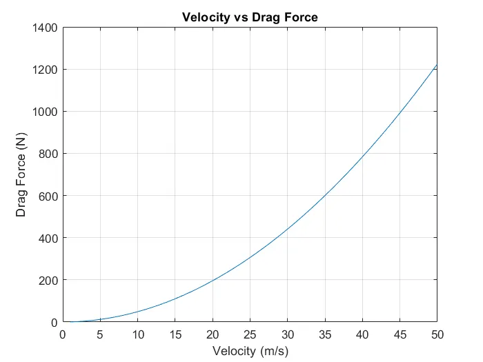
Figure 2 -