Week 8 - Natural Convection-II

AIM : To Simulate cooling of Low Voltage Panel using natural convection heat transfer in Ansys ICEPAK.

OBJECTIVES :

• Build the model as per the provided information.
• Create optimal meshing for the model.
• Setup the model for the Analysis.
• Run the simulation and Post Process the results.

INTRODUCTION :

Low voltage panels are used to distribute power from the main power source to different branches. It is a component of an electrical distribution system that divides an electrical power feed into branch circuits while providing a protective fuse or circuit breaker for each circuit in a common enclosure.

Low voltage (LV) panels are most common across all the industries and one of the more common special requirement which need to be designed in accordance with safety standards prevailing. An electrical panel is that the combination of protection and switch devices assembled in one or a lot of adjacent compartments.

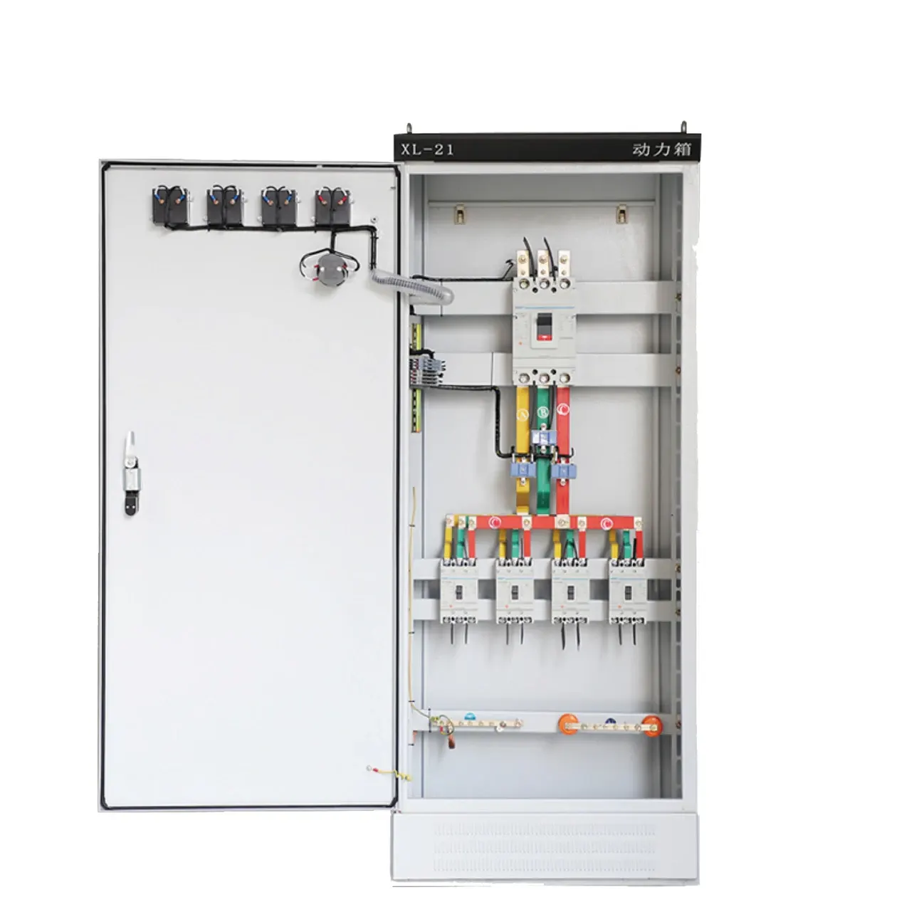
Main Components of a Low Voltage panel -

Enclosure - It houses all the components of the panel. It mount switches, knobs and displays and also to prevent electrical shock to equipment users. To safeguard the contents from the environment. Generally, it is made up of steel material and painted to avoid from rusting.

Circuit Breaker is an automatically operated electrical switch designed to protect an electric circuit from damage caused by excess current from an overload or short circuit. Its basic function is to interrupt current flow after a fault is detected. Unlike a fuse, which operates once and then must be replaced, a circuit breaker can be reset (either manually or automatically) to resume normal operation.

Busbars are used to distribute power between different circuit breakers. It is generally made up of material with high electrical conductivity. Also, a cross-section of the busbar is made larger to reduce the electrical resistance.

Cables are used to supply power to the different components from circuit breakers.

STEPS / PROCEDURE :

1) Creating Geometry and Assigning their Properties & Boundary Conditions

For the our project we have given the following data for the Low Voltage panel setup -

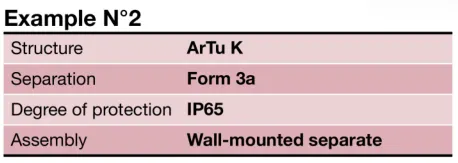
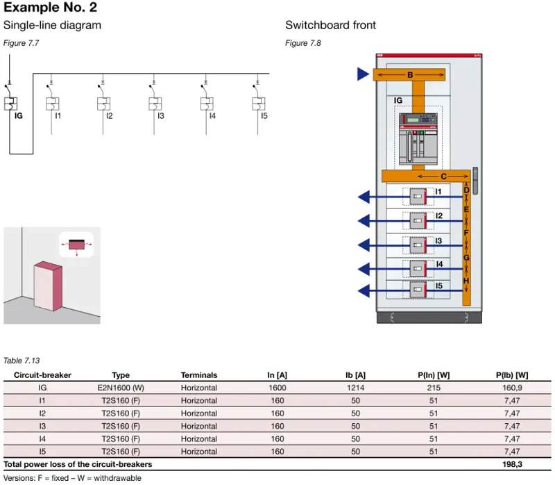
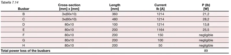
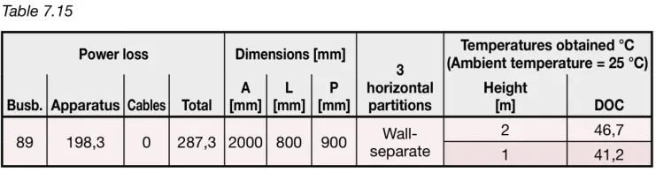
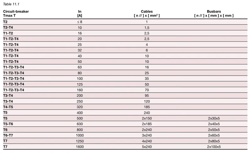
(Data sheet Reference source - https://new.abb.com/products/GD6002/artu-k )

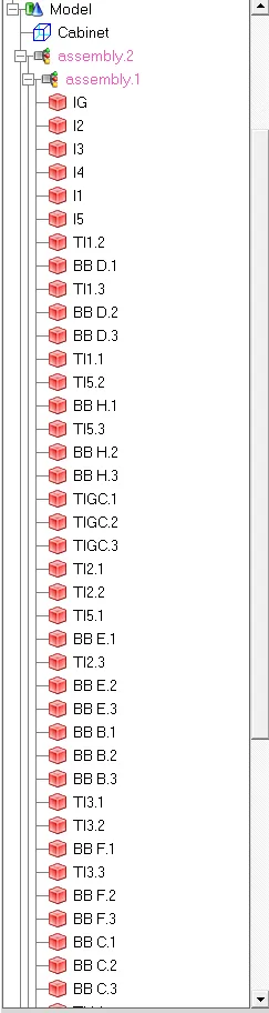
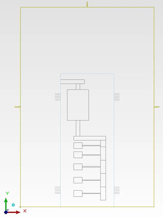
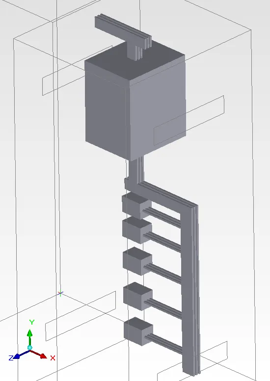
As the all Circuit Breakers are having 3-terminals ports, therefore the model assembly can be visaulized as this.

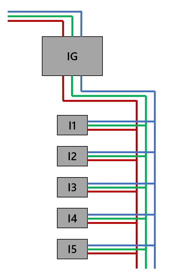
Following are the Geometry creation and assignments as given in the Case -

Enclosure -

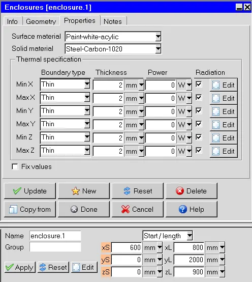
Cabinet -

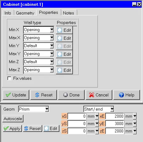
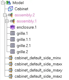
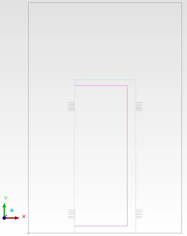
Circuit Breakers and there terminals-

IG-

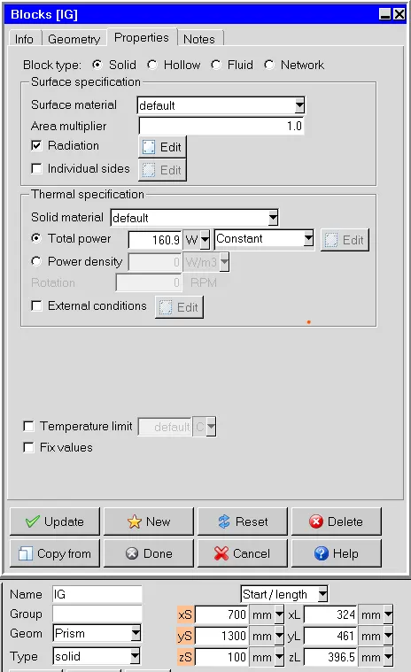
I1-

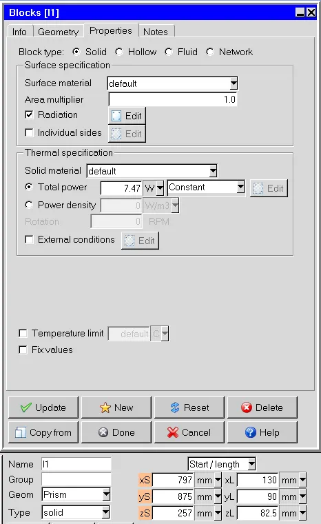
I2, I3, I4 and I5 are similiar to I2.

Busbars -

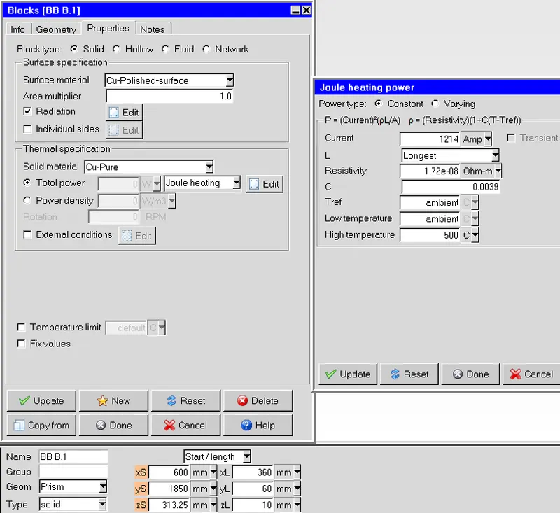
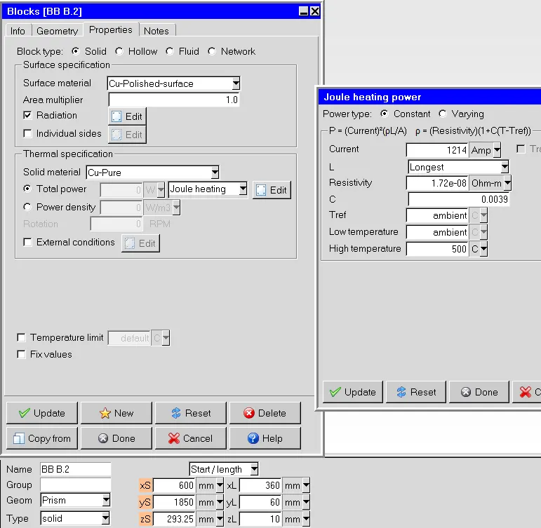
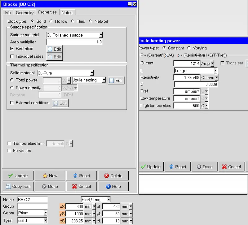
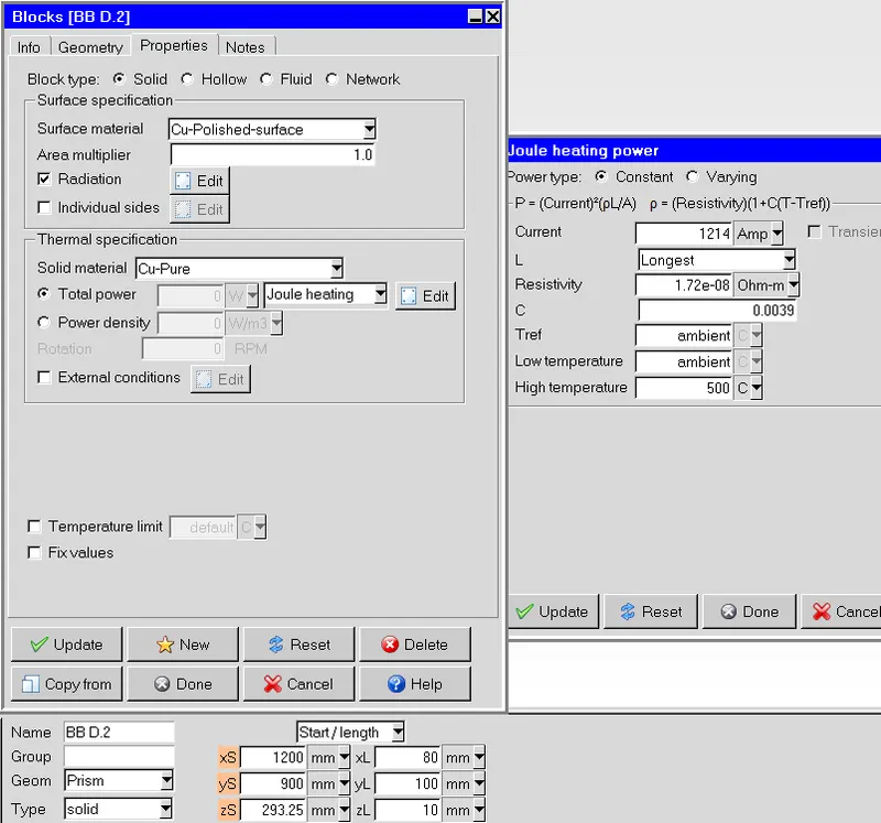
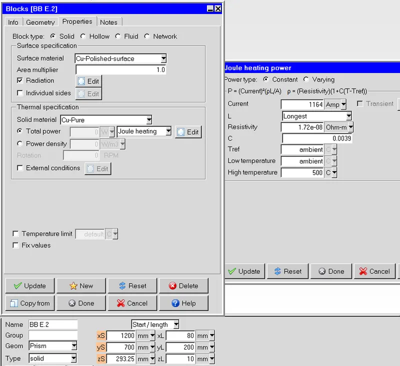
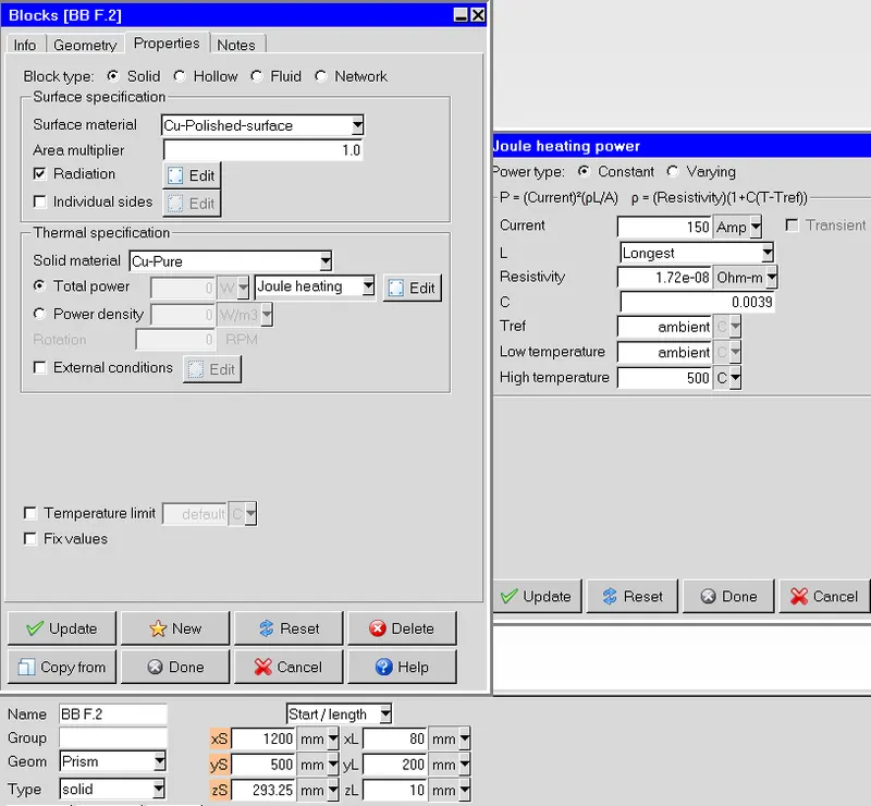
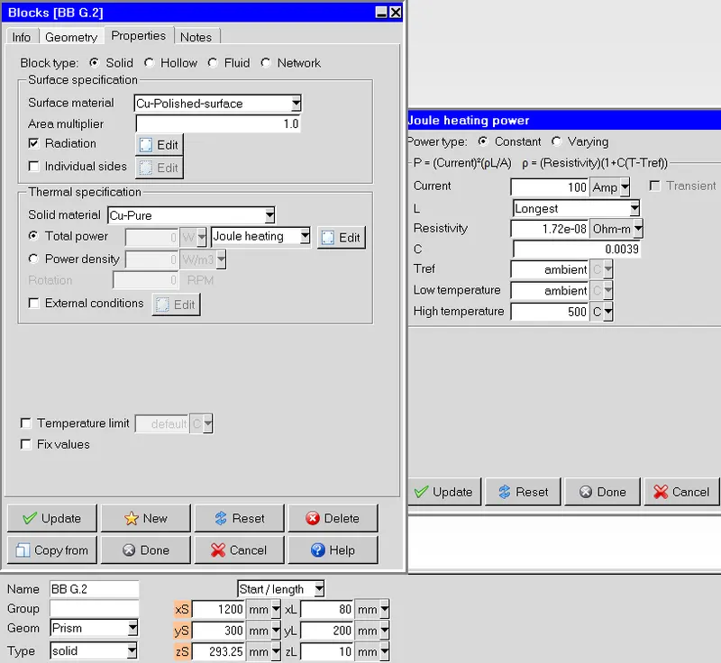
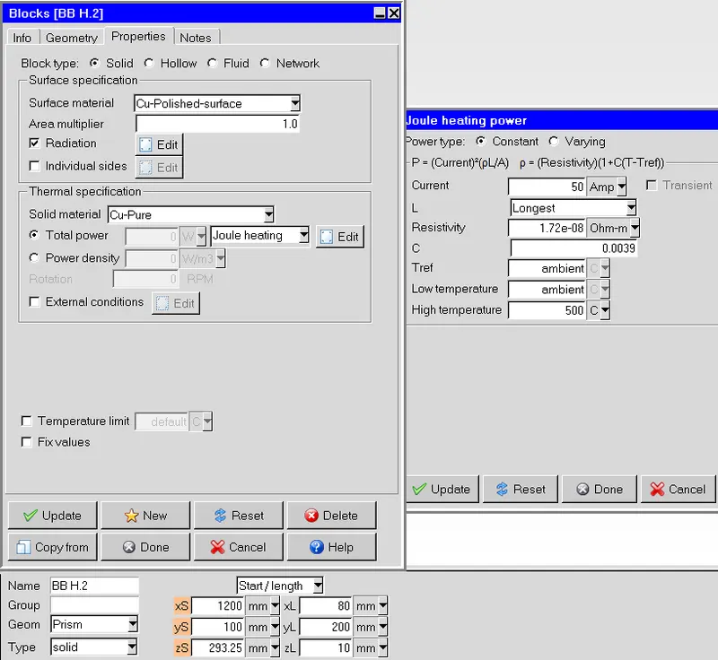
Terminals -

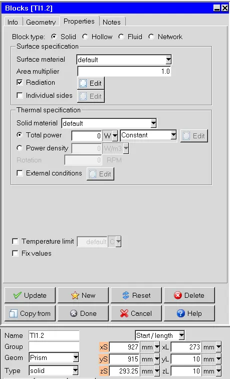
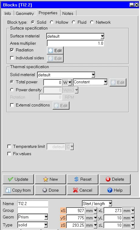
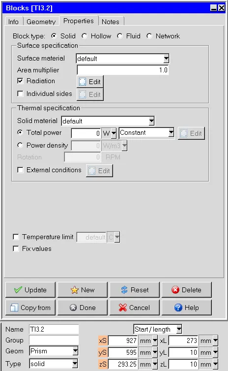
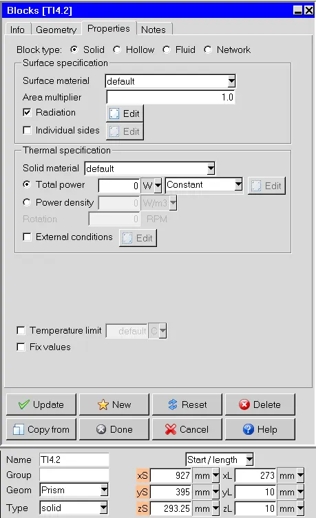
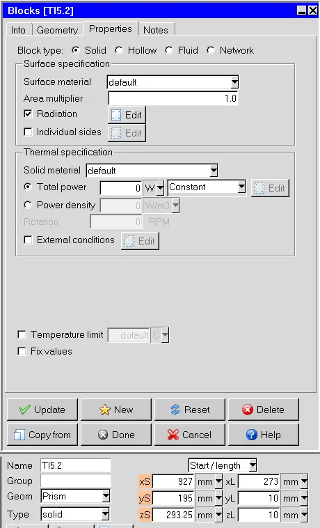
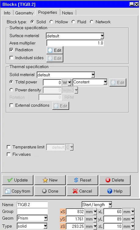
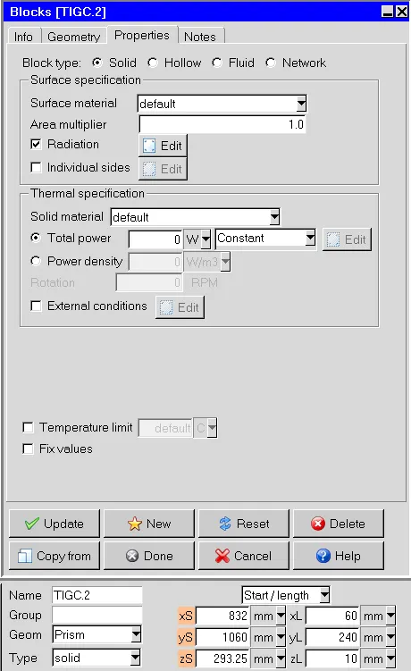
The System setup of Low Volatage control panel as follows -

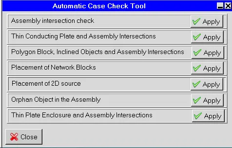
Case check tool in Macros options-

4) MESHING

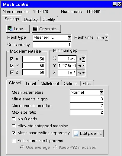
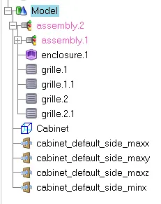
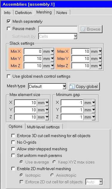
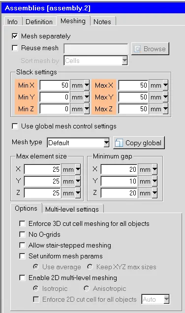
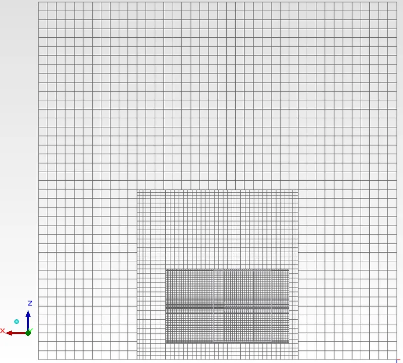
We have created a non-conformal mesh assembly accross the component assembly. To have fine mesh near to the components and coarser mesh across the enclosure and its ambient.

Following is setting used for global mesh and the assembly mesh settings -

5) Mesh Quality Parameters

Following is the surface mesh of the Case Setup -

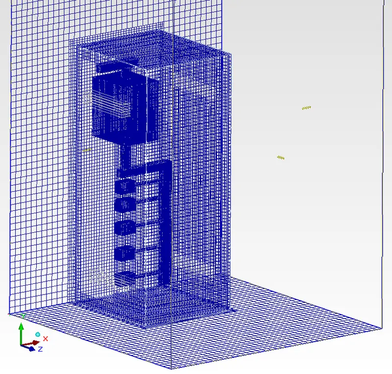
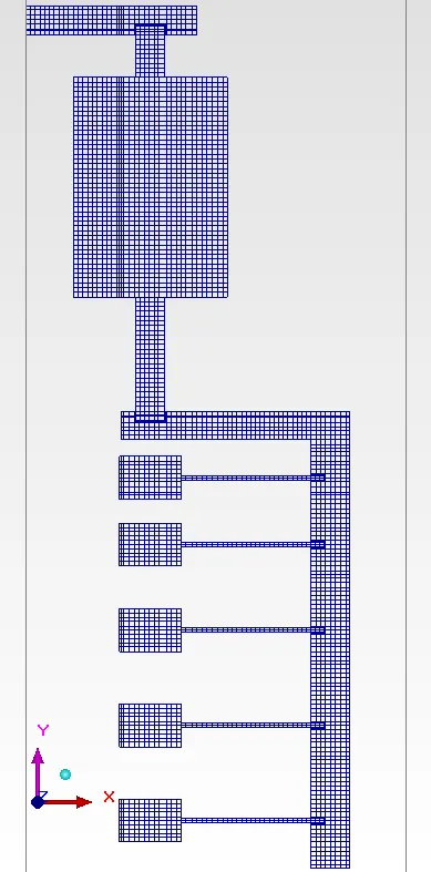
Following is the visualising the mesh inside the cabinet-

- Cut plane of XY plane at 50% of the cabinet in Z-direction from origin (Top Plane)

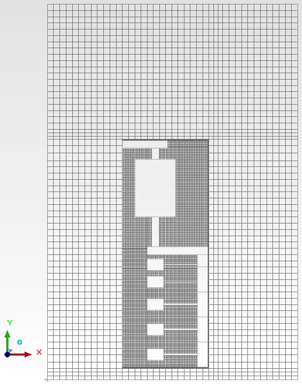
- Cut plane of YZ plane at 50% of the cabinet in X-direction from origin (Front Plane)

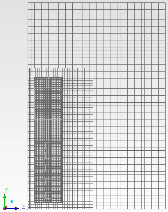
- Cut plane of XZ plane at 50% of the cabinet in Y-direction from origin (Right Plane)

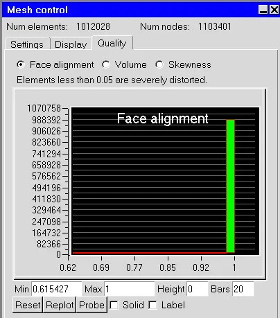
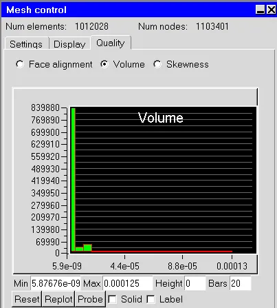
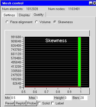
We can the mesh quality is very satisfied. 90% of the mesh cell are lying on good quality range.

Solver Settings -

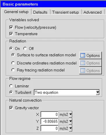
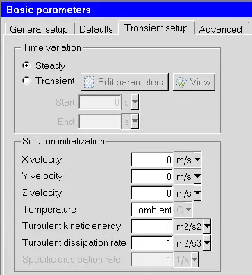
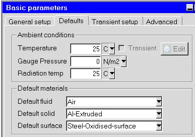
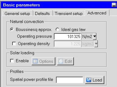
Gravity option is turned on since the majority of the fluid flow and heat transfer due to natural convection.

Inorder to capture the turbulence flow conditions we have chosen two equation model option i.e. K-epsilon turbulance model. Since, vortices / turbluence plays major roll in the heat transfer and therefore cooling.

Radiation solver has been enabled because in natural convection radiation cooling a play role in heat transfer.

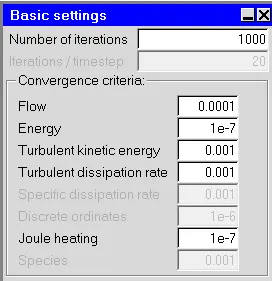
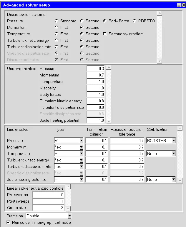
The solver setting majorily have kept default. and the discretization schemes are kept 2nd order in-order to more accuracy after running first cut simulation 1st order schemes.

POST PROCESSING :

Outputs

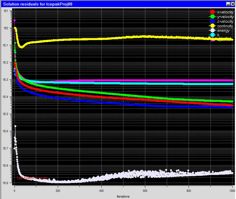
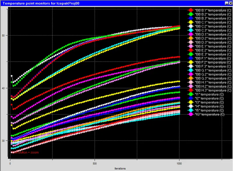
Residuals and Monitor Points -

Temperature Contours -

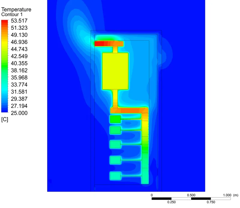
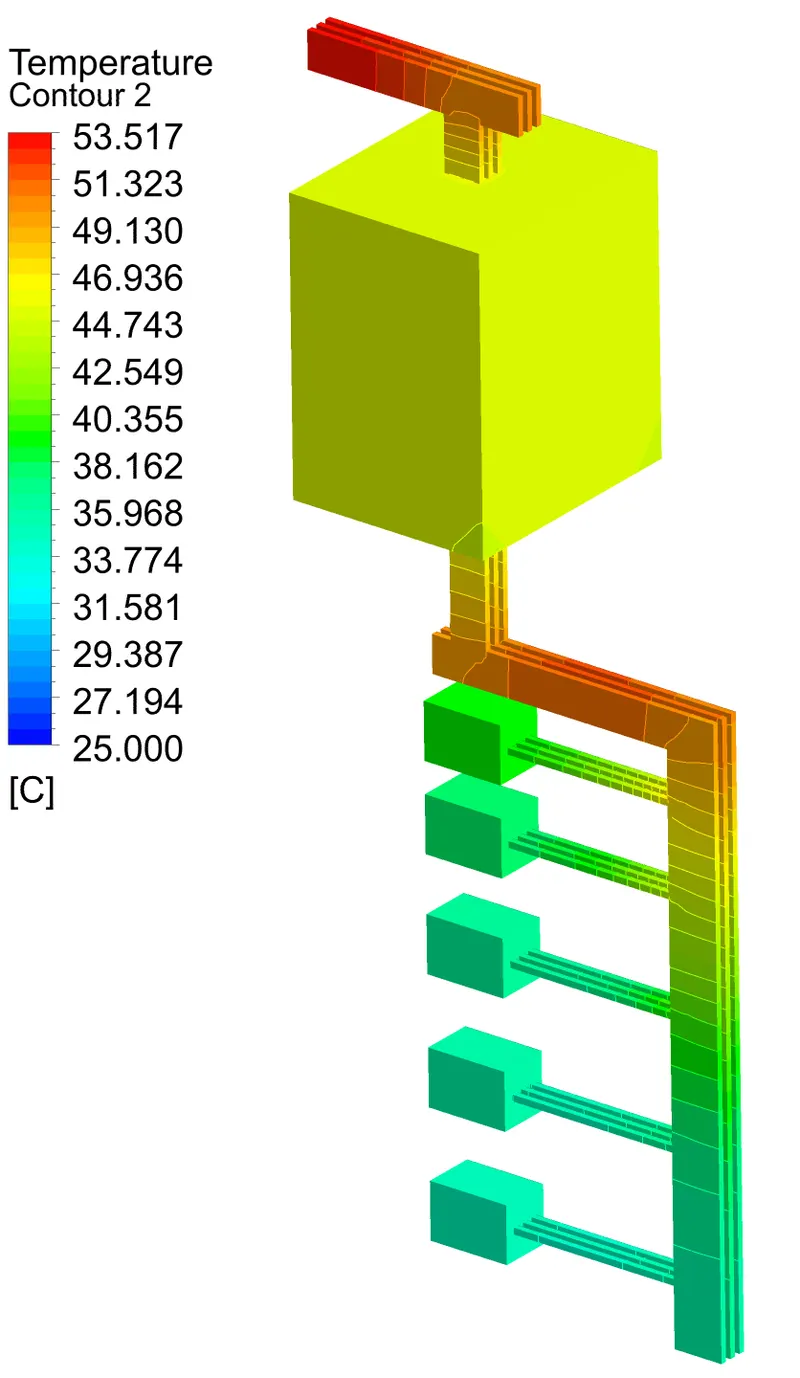
From the above temperature contours we can see the temperatures across various circuit breakers.

We can also notice the temperatures at busbars and cables due to joule heating.

In the first temperature contour, one can also observe the volumetric air temperature gradient from bottom to top.

Observing circuit breaker busbar B and IG, there is maximum temperature.

we can see that the components exposed infront of the inlet vent, are having lesser temperature than others.

Contour and Streamline Visulization of Velocity of the fluid -

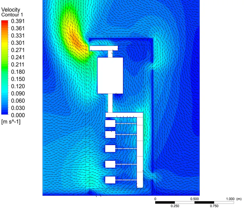
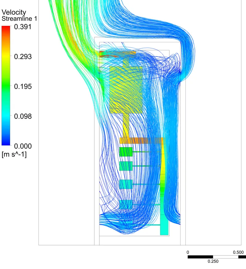
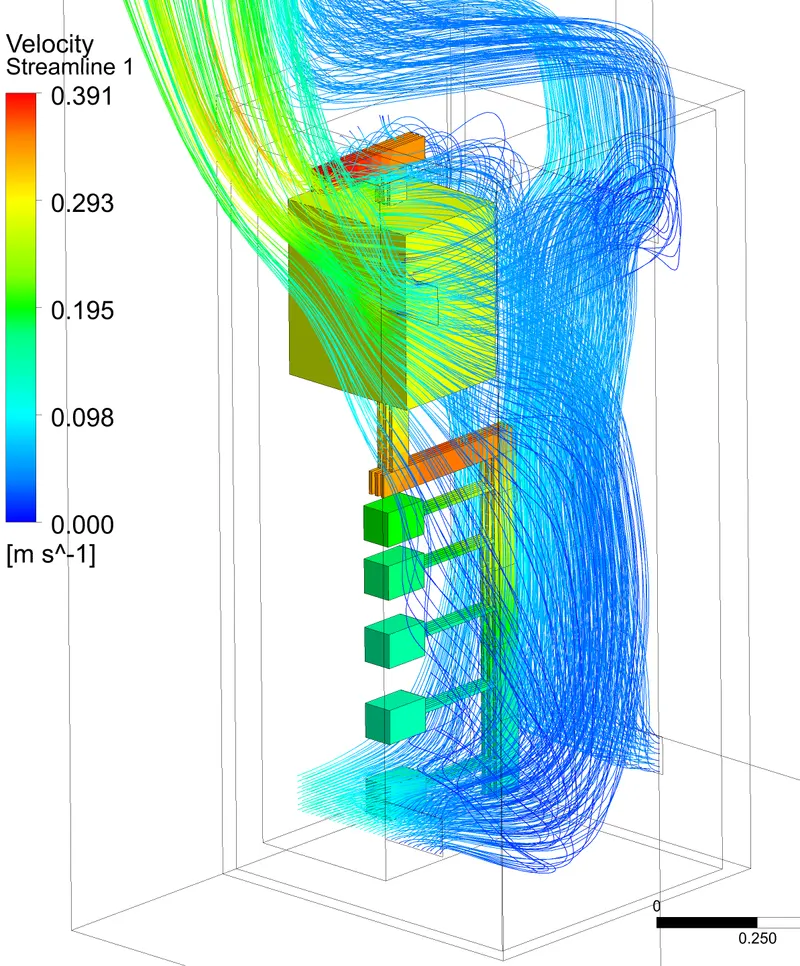
From the above countour we can see the velocity magnitude, velocity vector and streamlines across the cabinet.

We can see the air flow circulation from bottom to the top due the buoyancy effect because of rise in the temperature.

Appx. Max 0.39 m/s velocity of the air is attained as seen in the contour due to natural convection.

RESULTS :

The Following are the results of the simulation, generated simulation report from the ICEPAK software Showing Various characteristic values of the simulation and the max. temperatures of the different bodies acting in the simulation -

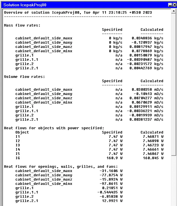
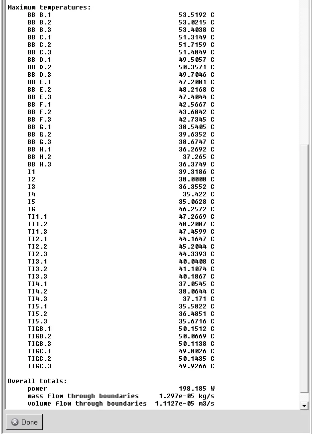
The maximum temperature within the computational domain is 53.5192 Deg.C. at the Busbar B due to joule heating.
The maximum air velocity within the computational domain is 0.39 m/s.

CONCLUSION :

We have successfully performed the simulation analysis for low voltage control panel, by creating the given geometry and suitable non-conformal mesh.

The solver was set up using suitable settings to incorporate the following physical phenomena: Joule heating, Natural convection, Turbulence, Radiation heat transfer.

We were able to generate required contours for temperature and speed. Also able post process streamline and animation of air circulation.

The following conclusions can be drawn based on the simulation results after running upto 100 iterations :

- We can see the temperatures attained are realistic and all the residuals are less than 10e-3 and continuity less than 10e-2.

- Maximum air velocity within the computational domain is 0.39 m/s.

The accuracy of the solution can be improved by refining the meshing and better by running the simulation for more no. of iterations, as currently the solution is partially stablize.