Mid-Term Project - Solving the steady and unsteady 2D heat conduction problem (ITCFDUML&OF/Challenge/Week5.1)

AIM - To write a Program in MATLAB for 2D Heat Conduction to study Steady state analysis & Transient State Analysis.

OBJECTIVE -

• Solving the steady and unsteady 2D heat conduction problem
• The Steady-state analysis, should be done by the following Iterative solvers - Jacobi, Gauss-siedel and SOR(Successive Over Relaxation) methods
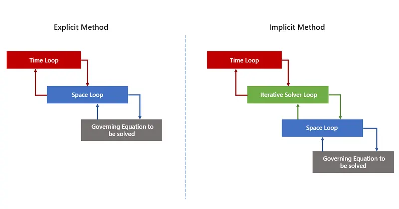
• The Transient State Analysis, is to be solved by the Expicit Method and Impicit Method
• Implcit equations must be solved via these iterative solvers - Jacobi, Gauss-siedel and SOR.

DETAILS AND CONSIDERATION -

• Consider the square plate of metal, of dimesions 1m x 1m.
• Temperatures at the boundaries of the plate,

Top Boundary = 600 K

Bottom Boundary = 900 K

Left Boundary = 400 K

Right Boundary = 800 K

• Thermal Diffusivity of the plate, `alpha` = 1.11e-4 `m^2`/s (Copper)
• Absolute error criteria is 1e-4
• Initial Condition, taking Initial temperature of nodes within the boundaries = 300K

THEORY -

Heat conduction (or thermal conduction) in general is the movement of heat from one object to another one that has different temperature when they are touching each other. Or the movement of heat from one end to the other positions/points on an object.

The Fourier's law of heat conduction states that the rate of heat transfer through a material is proportional to the negative gradient in the temperature and to the area, at right angles to that gradient, through which the heat flows.

`q= Q/A = -kgradT`

its one-dimensional form -

`q = -kA (dT)/(dx)`

where, q = the local heat flux density, (W/`m^2`)

k = the material's thermal conductivity, (W/(m.K))

`gradT` = the temperature gradient, (K/m)

Q = Heat Energy (W), A = Area(`m^2`)

2D Heat Conduction Equation -

1. Steady-State Heat Conduction -

A system/process is said to be in steady state condition, when the characteristic variables of the system/process does not changes with time. Steady-State Heat Conduction means, the temperature across the domain does not changes with time. That means, the Temperature is only the function of space(position) and not the function time.

The Steady-State heat conduction for 2D analysis is can be decuced as shown below -

`(del^2T)/(delx^2)+(del^2T)/(dely^2) = 0`

2. Transient or unsteady-state Heat Conduction -

A system/process is said to be in transient condition, whose characteristic variables of the system/process changes with time. Transient Heat Conduction means, the temperature across the domain changes with time. The Temperature is the function of space(position) and time.

`(delT)/(delt)+alpha((del^2T)/(delx^2)+(del^2T)/(dely^2)) = 0`

Where, `alpha` is thermal diffusivity

Discretization for Numerical Solution -

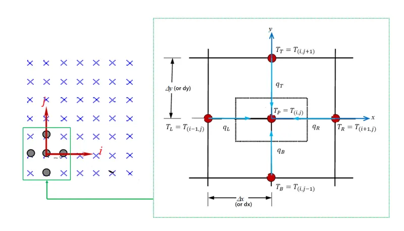
Here, `T_T =` T_Top, `T_B =` T_Bottom,

`T_L =` T_Left, `T_R =` T_Right

1. Discretized governing equation for the Steady-State 2D Heat Conduction -

`(del^2T)/(delx^2)+(del^2T)/(dely^2) = 0`

`implies (T_(i+1,j) - 2(T_(i,j)) +T_(i-1,j) )/(dx^2) + (T_(i,j+1) - 2(T_(i,j)) +T_(i,j-1) )/(dy^2) = 0`

`implies (T_(R) - 2(T_P) +T_(L) )/(dx^2) + (T_(T) - 2(T_(P)) +T_(B) )/(dy^2) = 0`

`implies T_P = (dy^2)/(2*(dx^2 + dy^2))*(T_R+T_L) + (dx^2)/(2*(dx^2 + dy^2))*(T_T+T_B)`

Considering `K_X = (dy^2)/(2*(dx^2 + dy^2))` and `K_Y = (dx^2)/(2*(dx^2 + dy^2))`

Therefore,

` T_P = K_X*(T_R+T_L) + K_Y*(T_T+T_B)`

2. Discretized governing equation for the Transient or Unsteady-State 2D Heat Conduction -

`(delT)/(delt)+alpha((del^2T)/(delx^2)+(del^2T)/(dely^2)) = 0`

`implies (T_(i,j)^(n+1)-T_(i,j)^(n))/(dt) + alpha*((T_(i+1,j) - 2(T_(i,j)) +T_(i-1,j) )/(dx^2) + (T_(i,j+1) - 2(T_(i,j)) +T_(i,j-1) )/(dy^2)) = 0`

Now the variable at current time step (i.e. at n) is showned by suffix of 'O' representing Old. and for the next time step (i.e. n+1) is by suffix of 'N'

`implies (T_(NP)-T_(OP))/(dt) + alpha*((T_(OR) - 2(T_(OP)) +T_(OL) )/(dx^2) + (T_(OT) - 2(T_(OP)) +T_(OB) )/(dy^2)) = 0`

`implies T_(NP)= T_(OP) + alpha*dt*((T_(OR) - 2(T_(OP)) +T_(OL) )/(dx^2) + (T_(OT) - 2(T_(OP)) +T_(OB) )/(dy^2)) `

Considering `K_(XT) = (alpha*dt)/(dx^2)` and `K_(YT) = (alpha*dt)/(dy^2)`

Explicit Equation -

` T_(NP)= T_(OP) + K_(XT)*(T_(OR) - 2(T_(OP)) +T_(OL)) + K_(XT)*(T_(OT) - 2(T_(OP)) +T_(OB) ) `

Implicit Equation -

` T_(NP)= T_(OP) + K_(XT)*(T_(NR) - 2(T_(NP)) +T_(NL)) + K_(XT)*(T_(NT) - 2(T_(NP)) +T_(NB) ) `

` implies T_(NP)= (T_(OP) + K_(XT)*(T_(NR)+T_(NL)) + K_(XT)*(T_(NT)+T_(NB)))/(1+2K_(XT)+2K_(YT)) `

Iterative Solvers -

1.Jacobi method: The Jacobi iteration method is employed on a system of linear equations for which a unique solution can be obtained and the main diagonal of the coefficient matrix has no zeros such that with every subsequent iteration, the values of the main diagonal elements are replaced by newly guessed values until a state of convergence is not achieved.

2.Gauss-seidel method: Similar to the Jacobi iteration method, the Gauss-seidel iteration method can be employed on a system of linear equations that has a unique solution and the leading diagonal of the coefficient matrix contains non-zero terms, however, the values along the main diagonal are replaced during the same iteration such that values to be computed at a given location that depend on them can utilise the newly guessed values unlike with Jacobi where the same process happens simultaneously. Therefore, the Jacobi iteration method is known as method of simultaneous replacements and the Gauss-seidel method as method of successive replacements.

3.Successive Over Relaxation iteration method: Also in short as SOR method can be considered as an extrapolation of the Gauss-seidel method such that a weighted average is utilised between the previous iteration and the newly computed value in an attempt to improve the performance of the base solver i.e., the Gauss-seidel method, by achieving a faster rate of convergence. There are, however, limitations to the value of the weighted average (also called as the extrapolation factor) beyond which possibilities of convergence become difficult.

THERMAL DIFFUSIVITY AND CFL CRITERIA -

The Thermal Diffusivity (`alpha`) in these type of problem is also an important factor the solution, as it is realated to the CFL Criteria show below,

`CFL = (alpha*dt)*((1/dx^2)+(1/dy^2))` or `dt = (CFL*dx^2*dy^2)/(alpha*(dx^2+dy^2))`

Thermal Diffusivity is inter-related with the dt, dx and the CFL number. Now for the material's thermal difussivity there will be a otimum CFL i.e. optimum value of dt, dx and dy. For the smaller value value of the `alpha` the size of dt will higher inorder to maintain stability i.e. here CFL no., but it reduces the accuracy of the solution, and for the larger value of `alpha` the size of dt will be small for the optimum CFL, but it can increase the simulation time. Since, the implicit method is unconditionally stable at any value of time step, still the CFL condtion can be used in order to determine the optimum 'dt' inorder to maintain time accuracies.

CODING LOGIC -

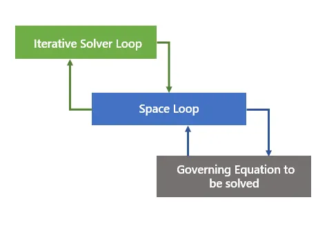
1. For Steady-State Heat Conduction

2. For Transient or Unsteady-State Heat Conduction

PROGRAM -

Following is the Main Function of the CODE for the 2 Heat Conduction for steady and unsteady state -

%   --------------------------------------------------------------- 2D HEAT CONDUCTION ---------------------------------------------------------------

% Domain 1m x 1m

% Boundary Condition - 
%
%       Top BC =  600K
%    Bottom BC =  900K
%      Left BC =  400K
%     Right BC =  800K

% Error tolerance or convergence residual criteria = 1e-4
clear all;
close all;
clc;


L = 1;      % Domain length (Same in both direction)
nx = 31;    % no. of nodes in X directions
ny = nx;    % no. of nodes in Y directions

x = linspace(0,L,nx);
y = linspace(0,L,ny);
[X,Y] = meshgrid(nx,ny);

dx = L/(nx-1);     % Space Step size in x-direction
dy = L/(ny-1);     % Space Step size in y-direction

tol = 1e-4;

% Creating Grid with assumed initial condition
T = 300*ones(nx,ny);

% Boundary Conditions
T(1, :) = 600;      % Top 
T(ny, :) = 900;     % Bottom
T(:, 1) = 400;      % Left
T(:, nx) = 800;     % Right

T(1,1)   = (400+600)/2;
T(1,ny)  = (800+600)/2;
T(nx,1)  = (900+400)/2;
T(nx,ny) = (900+800)/2;

% for The Steady-state Analysis

Kx = (dy^2)/(2*(dx^2 + dy^2));
Ky = (dx^2)/(2*(dx^2 + dy^2));

% Considerations for The Transient Analysis

alpha = 1.11*(10^(-4));     % Thermal Diffusivity of Aluminium

nt = 1000;
cfl = 0.5;
dt = (cfl*dx^2*dy^2)/(alpha*(dx^2+dy^2));
%dt = 6.25;
%CFL = (alpha*dt)*((1/dx^2)+(1/dy^2))
t = nt*dt;

Kxt = alpha*(dt/(dx^2));
Kyt = alpha*(dt/(dy^2));

z=cos(pi/nx-1)+cos(pi/ny-1);
omega = 4/(2+sqrt(4-z^2));

fprintf(' nttttt The 2D Heat Condition Problem n ');
fprintf(' nt Choose the study Approach from the following - n');
fprintf(' ntt 1 - Steady-State Analysis via Jacobi iterative solver ');
fprintf(' ntt 2 - Steady-State Analysis via Gauss-Siedel iterative solver ');
fprintf(' ntt 3 - Steady-State Analysis via  Successive Over Relaxation with Gauss-Seidel solver ');
fprintf(' ntt 4 - Transient Analysis with explicit method ');
fprintf(' ntt 5 - Transient Analysis with implicit via Jacobi iterative solver ');
fprintf(' ntt 6 - Transient Analysis with implicit via Gauss-Siedel iterative solver ');
fprintf(' ntt 7 - Transient Analysis with implicit via Successive Over Relaxation with Gauss-Seidel solver n');
choice = input('n     Enter your choice = ');

To = T;         % For the old value at iterative solvers ( provides value of previous iteration)
Tpast = T;      % Tpast is the matrix for the values at previous timestep


%--------------------------------------------------------------------------------------
% 1 - Steady-State Analysis via Jacobi iterative solver
%--------------------------------------------------------------------------------------
if choice == 1
    tic;
    error = 9e9;
    iter = 0;
    while(error > tol)
        
        for i = 2 : nx-1
            for j = 2 : ny-1
                
                T(i,j) = Kx*(To(i-1,j) + To(i+1,j)) + Ky*(To(i,j-1) + To(i,j+1));
                
            end
        end
        error = max(max(abs(To-T)));
        iter = iter + 1;
        
        To = T;
        
    end
    
    figure(1)
        contourf(x,y,T,50,':'); %contourf(X,Y,T);
    	colormap(turbo(50));
    	mtitle = sprintf('Steady-State 2D heat Conduction via Jacobi Iterative Solver');
        tsim = toc;
    	stitle = sprintf(' Iterations = %d , Simulation Time = %.4f',iter,tsim);
    	title(mtitle,stitle);
    	xlabel(' X  (1 metre)');     ylabel(' Y (1 metre)');
    	set(gca, 'Ydir', 'reverse');
    	cb = colorbar;
    	cb.Title.String ='Temp. (in K)';
    	cb.Title.Position(1,1);
   
    fprintf(' nt Steady-State Analysis via Jacobi iterative solver ');
    fprintf(' nntt Space Step Size = %.4f',dx);
    fprintf(' ntt CFL Criteria, Courant No. = %.1f ',cfl);
    fprintf(' ntt No. of Time Steps = %d ',nt);
    fprintf(' ntt Time Step Size  = %.4f Secs', dt)
    fprintf(' ntt Simulating for time  = %.4f Secs',t);
    fprintf(' ntt No. of Iteration = %d ',iter);
    fprintf(' ntt Time taken for simulation = %.4f Secs n',tsim);


            
%--------------------------------------------------------------------------------------            
% 2 - Steady-State Analysis via Gauss-Siedel iterative solver
%--------------------------------------------------------------------------------------
elseif choice == 2
    tic;
    error = 9e9;
    iter = 0;
    while(error > tol)
        
        for i = 2 : nx-1
            for j = 2 : ny-1
                
                T(i,j) = Kx*(T(i-1,j) + To(i+1,j)) + Ky*(T(i,j-1) + To(i,j+1)); 

                
            end
        end
        error = max(max(abs(To-T)));
        To = T;
        iter = iter + 1;
    end
    
    figure(2)
        contourf(x,y,T,50,':'); %contourf(X,Y,T);
    	colormap(turbo(50));
    	mtitle = sprintf('Steady-State 2D heat Conduction via Gauss-Siedel Iterative Solver');
        tsim = toc;
    	stitle = sprintf(' Iterations = %d , Simulation Time = %.4f',iter,tsim);
    	title(mtitle,stitle);
    	xlabel(' X  (1 metre)');     ylabel(' Y (1 metre)');
    	set(gca, 'Ydir', 'reverse');
    	cb = colorbar;
    	cb.Title.String ='Temp. (in K)';
    	cb.Title.Position(1,1); 
    
    fprintf(' nt Steady-State Analysis via Gauss-Siedel iterative solver ');
    fprintf(' nntt Space Step Size = %.4f',dx);
    fprintf(' ntt CFL Criteria, Courant No. = %.1f ',cfl);
    fprintf(' ntt No. of Time Steps = %d ',nt);
    fprintf(' ntt Time Step Size  = %.4f Secs', dt)
    fprintf(' ntt Simulating for time  = %.4f Secs',t);
    fprintf(' ntt No. of Iteration = %d ',iter);
    fprintf(' ntt Time taken for simulation = %.4f Secs n',tsim);
    
%--------------------------------------------------------------------------------------
% 3 - Steady-State Analysis via Successive Over Relaxation with Gauss-Seidel solver
%--------------------------------------------------------------------------------------
elseif choice == 3
    tic
    error = 9e9;
    iter = 0;
    while(error > tol)
        
        for i = 2 : nx-1
            for j = 2 : ny-1
                
                T(i,j) = omega*Kx*(T(i-1,j) + To(i+1,j)) + omega*Ky*(T(i,j-1) + To(i,j+1)) + (1-omega)*To(i,j);   
                
            end
        end
        error = max(max(abs(To-T)));
        To = T;
        iter = iter + 1;
    end
    
    figure(3)
        contourf(x,y,T,50,':'); %contourf(X,Y,T);
    	colormap(turbo(50));
    	mtitle = sprintf('Steady-State 2D heat Conduction via Successive Over Relaxation with Gauss-Seidel ');
        tsim = toc;
    	stitle = sprintf(' Iterations = %d , Simulation Time = %.4f',iter,tsim);
    	title(mtitle,stitle);
    	xlabel(' X  (1 metre)');     ylabel(' Y (1 metre)');
    	set(gca, 'Ydir', 'reverse');
    	cb = colorbar;
    	cb.Title.String ='Temp. (in K)';
    	cb.Title.Position(1,1);     
    
    fprintf(' nt Steady-State Analysis via  Successive Over Relaxation with Gauss-Seidel solver ');
    fprintf(' nntt Space Step Size = %.4f',dx);
    fprintf(' ntt Relaxation Factor = %.4f',omega);
    fprintf(' ntt CFL Criteria, Courant No. = %.1f ',cfl);
    fprintf(' ntt No. of Time Steps = %d ',nt);
    fprintf(' ntt Time Step Size  = %.4f Secs', dt)
    fprintf(' ntt Simulating for time  = %.4f Secs',t);
    fprintf(' ntt No. of Iteration = %d ',iter);
    fprintf(' ntt Time taken for simulation = %.4f Secs n',tsim);  

%--------------------------------------------------------------------------------------
% 4 - Transient Analysis with explicit method
%--------------------------------------------------------------------------------------
elseif choice == 4
    tsim = 0;
    iter = 0;
    ct = 1; 
    for st = 1:nt % Time Loop
        tic;
        error = 9e9;
        To = Tpast;
            
            for i = 2 : nx-1
                for j = 2 : ny-1
                    
                    T(i,j) = To(i,j) + Kxt*(To(i+1,j)-(2*To(i,j))+To(i-1,j)) + Kyt*(To(i,j+1)-(2*To(i,j))+To(i,j-1));
                    
                end
            end
        iter = iter+1;
        time = st*dt;
        figure(4)
        contourf(x,y,T,50,':'); 
        %surf(x,y,T);
    	colormap(turbo(50));
    	mtitle = sprintf(' Transient 2D heat Conduction by Explicit method ');
        tsim = tsim + toc;
    	stitle = sprintf('TimeStep = %.4f , Simulation Time = %.4f',time,tsim);
    	title(mtitle,stitle);
    	xlabel(' X  (1 metre)');     ylabel(' Y (1 metre)');
    	set(gca, 'Ydir', 'reverse');
    	cb = colorbar;
    	cb.Title.String ='Temp. (in K)';
    	cb.Title.Position(1,1); 
        pause(0.01);
        M(ct) = getframe(gcf);          % by getframe it Captures figure as movie frame
        ct = ct+1;
        
        Tpast = T;
    end
   
    fprintf(' nt Transient Analysis with explicit method ');
    fprintf(' nntt Space Step Size = %.4f',dx);
    fprintf(' ntt CFL Criteria, Courant No. = %.1f ',cfl);
    fprintf(' ntt No. of Time Steps = %d ',nt);
    fprintf(' ntt Time Step Size  = %.4f Secs', dt)
    fprintf(' ntt Simulating for time  = %.4f Secs',t);
    fprintf(' ntt No. of Iteration = %d ',iter);
    fprintf(' ntt Time taken for simulation = %.4f Secs n',tsim);
    
    movie(M);   % Play recorded movie frames
    video = VideoWriter('Transient 2D heat Conduction by Explicit method.avi','Motion JPEG AVI'); 
    % Write video files and assigning video file name and video format
    open(video);            % Open file for writing video data
    writeVideo(video,M);    % Write video data to file
    close(video);           % Close file after writing video data
  
%--------------------------------------------------------------------------------------
% 5 - Transient Analysis with implicit via Jacobi iterative solver
%--------------------------------------------------------------------------------------
elseif choice == 5
    tsim = 0;
    iter = 0;
    ct = 1;
    for st = 1:nt
        tic;
        error = 9e9;
        To = Tpast; 

        while(error > tol)
            
            for i = 2 : nx-1
                for j = 2 : ny-1
                    
                    T(i,j) = (Tpast(i,j) + Kxt*(To(i+1,j)+To(i-1,j)) + Kyt*(To(i,j+1)+To(i,j-1)))/(1+(2*Kxt)+(2*Kyt));
                    
                end
            end
            error = max(max(abs(To-T)));
            To = T;
            iter = iter + 1;
        end

        time = st*dt;
        figure(5)
        contourf(x,y,T,50,':'); 
    	colormap(turbo(50));
    	mtitle = sprintf('Transient 2D heat Conduction by Implicit method via Jacobi');
        tsim = tsim + toc;
    	stitle = sprintf(' TimeStep = %.4f , Simulation Time = %.4f',time,tsim);
    	title(mtitle,stitle);
    	xlabel(' X  (1 metre)');     ylabel(' Y (1 metre)');
    	set(gca, 'Ydir', 'reverse');
    	cb = colorbar;
    	cb.Title.String ='Temp. (in K)';
    	cb.Title.Position(1,1); 
        pause(0.01);
        M(ct) = getframe(gcf);          % by getframe it Captures figure as movie frame
        ct = ct+1;
        
        Tpast = T;
    end
   
    fprintf(' nt Transient Analysis with implicit via Jacobi iterative solver ');
    fprintf(' nntt Space Step Size = %.4f',dx);
    fprintf(' ntt CFL Criteria, Courant No. = %.1f ',cfl);
    fprintf(' ntt No. of Time Steps = %d ',nt);
    fprintf(' ntt Time Step Size  = %.4f Secs', dt)
    fprintf(' ntt Simulating for time  = %.4f Secs',t);
    fprintf(' ntt No. of Iteration = %d ',iter);
    fprintf(' ntt Time taken for simulation = %.4f Secs n',tsim);
    
    movie(M);   % Play recorded movie frames
    video = VideoWriter('Transient 2D heat Conduction with Implicit method via Jacobi.avi','Motion JPEG AVI'); 
    open(video);            % Open file for writing video data
    writeVideo(video,M);    % Write video data to file
    close(video);           % Close file after writing video data
    
%--------------------------------------------------------------------------------------
% 6 - Transient Analysis with implicit via Gauss-Siedel iterative solver
%--------------------------------------------------------------------------------------
elseif choice == 6
    tsim = 0;
    iter = 0;
    ct = 1; 
    for st = 1:nt
        tic;
        error = 9e9;
        To = Tpast; 

        while(error > tol)
            
            for i = 2 : nx-1
                for j = 2 : ny-1
                    
                    T(i,j) = (Tpast(i,j) + Kxt*(T(i-1,j)+To(i+1,j)) + Kyt*(T(i,j-1)+To(i,j+1)))/(1+(2*Kxt)+(2*Kyt));
                    
                end
            end
            error = max(max(abs(To-T)));
            To = T;
            iter = iter + 1;
        end

        time = st*dt;
        figure(6)
        contourf(x,y,T,50,':'); 
    	colormap(turbo(50));
    	mtitle = sprintf('Transient 2D heat Conduction by Implicit method via Gauss-Siedel');
        tsim = tsim + toc;
    	stitle = sprintf(' TimeStep = %.4f , Simulation Time = %.4f',time,tsim);
    	title(mtitle,stitle);
    	xlabel(' X  (1 metre)');     ylabel(' Y (1 metre)');
    	set(gca, 'Ydir', 'reverse');
    	cb = colorbar;
    	cb.Title.String ='Temp. (in K)';
    	cb.Title.Position(1,1); 
        pause(0.01);
        M(ct) = getframe(gcf);          % by getframe it Captures figure as movie frame
        ct = ct+1;
        
        Tpast = T;
    end
   
    fprintf(' nt Transient Analysis with implicit via Gauss-Siedel iterative solver ');
    fprintf(' nntt Space Step Size = %.4f',dx);
    fprintf(' ntt CFL Criteria, Courant No. = %.1f ',cfl);
    fprintf(' ntt No. of Time Steps = %d ',nt);
    fprintf(' ntt Time Step Size  = %.4f Secs', dt)
    fprintf(' ntt Simulating for time  = %.4f Secs',t);
    fprintf(' ntt No. of Iteration = %d ',iter);
    fprintf(' ntt Time taken for simulation = %.4f Secs n',tsim);
    
    movie(M);   % Play recorded movie frames
    video = VideoWriter('Transient 2D heat Conduction with Implicit method via Gauss-Siedel.avi','Motion JPEG AVI'); 
    open(video);            % Open file for writing video data
    writeVideo(video,M);    % Write video data to file
    close(video);           % Close file after writing video data

    
%--------------------------------------------------------------------------------------
% 7 - Transient Analysis with implicit via SOR-GS iterative solver
%--------------------------------------------------------------------------------------
elseif choice == 7
    
    tsim = 0;
    iter = 0;
    ct = 1; 
    
    for st = 1:nt
        tic;
        error = 9e9;
        To = Tpast; 
        
        while(error > tol)
            
            for i = 2 : nx-1
                for j = 2 : ny-1
                    
                    T(i,j) =  (1-omega)*To(i,j) + ((omega*Tpast(i,j)) + (omega*Kxt*(T(i-1,j)+To(i+1,j))) + (omega*Kyt*(T(i,j-1)+To(i,j+1))) )/(1+(2*Kxt)+(2*Kyt));
                    
                end
            end
            error = max(max(abs(To-T)));
            To = T;
            iter = iter + 1;
        end

        time = st*dt;
        figure(7)
        contourf(x,y,T,50,':'); 
    	colormap(turbo(50));
    	mtitle = sprintf('Transient 2D heat Conduction by Implicit method via SOR');
        tsim = tsim + toc;
    	stitle = sprintf(' TimeStep = %.4f , Simulation Time = %.4f',time,tsim);
    	title(mtitle,stitle);
    	xlabel(' X  (1 metre)');     ylabel(' Y (1 metre)');
    	set(gca, 'Ydir', 'reverse');
    	cb = colorbar;
    	cb.Title.String ='Temp. (in K)';
    	cb.Title.Position(1,1); 
        pause(0.01);
        M(ct) = getframe(gcf);          % by getframe it Captures figure as movie frame
        ct = ct+1;

        Tpast = T;
    end
   
    fprintf(' nt Transient Analysis with implicit via Successive Over Relaxation with Gauss-Seidel solver n');
    fprintf(' nntt Space Step Size = %.4f',dx);
    fprintf(' ntt Relaxation Factor = %.4f',omega);
    fprintf(' ntt CFL Criteria, Courant No. = %.1f ',cfl);
    fprintf(' ntt No. of Time Steps = %d ',nt);
    fprintf(' ntt Time Step Size  = %.4f Secs', dt)
    fprintf(' ntt Simulating for time  = %.4f Secs',t);
    fprintf(' ntt No. of Iteration = %d ',iter);
    fprintf(' ntt Time taken for simulation = %.4f Secs n',tsim);
    
    movie(M);   % Play recorded movie frames
    video = VideoWriter('Transient 2D heat Conduction with Implicit method via SOR.avi','Motion JPEG AVI'); 
    open(video);            % Open file for writing video data
    writeVideo(video,M);    % Write video data to file
    close(video);           % Close file after writing video data
    
%--------------------------------------------------------------------------------------
else
    fprintf(' n ttttInvalid Choice! Choose between Options 1 to 7 n');
    
end

OUTPUT -

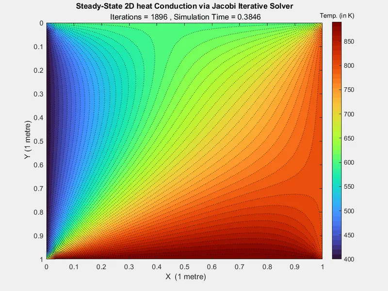
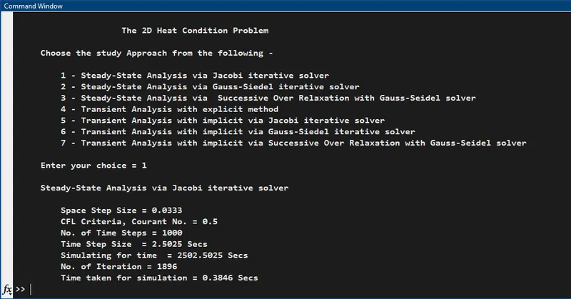
1. For Choice = 1, Steady-State Analysis via Jacobi iterative solver

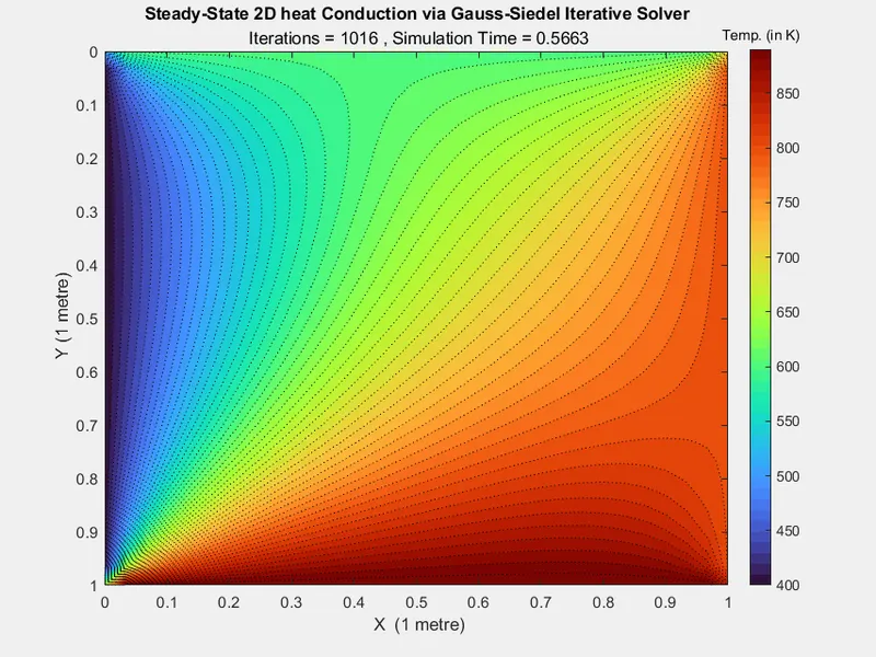
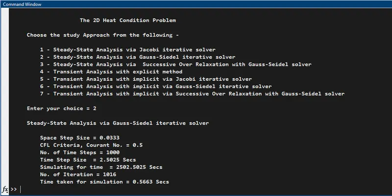
2. For Choice = 2, Steady-State Analysis via Gauss-Siedel iterative solver

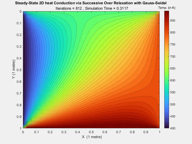
3. For Choice = 3, Steady-State Analysis via Successive Over Relaxation with Gauss-Seidel solver

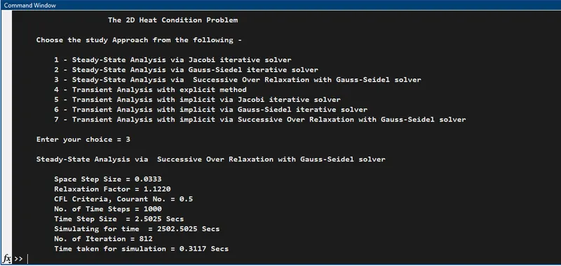
4. For Choice = 4, Transient Analysis with explicit method

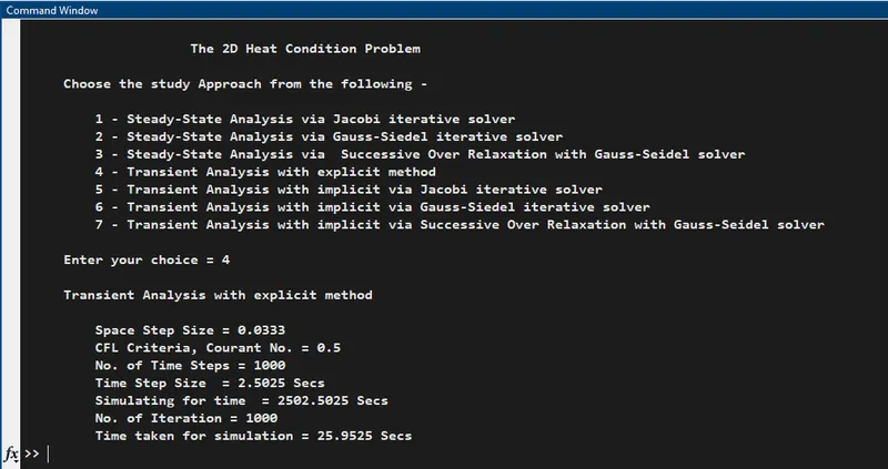
5. For Choice = 5, Transient Analysis with implicit via Jacobi iterative solver

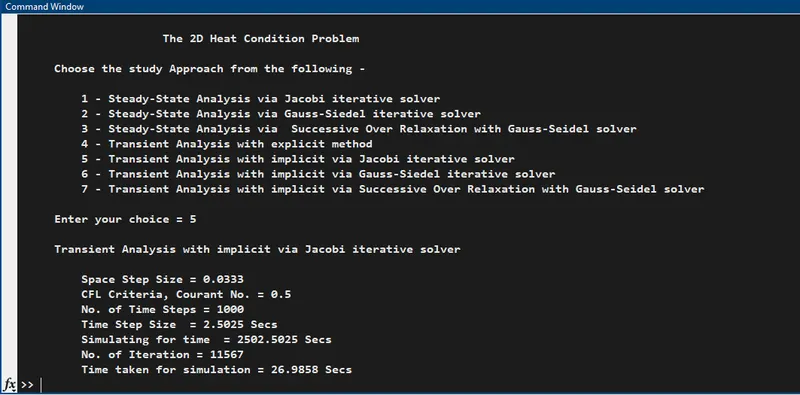
6. For Choice = 6, Transient Analysis with implicit via Gauss-Siedel iterative solver

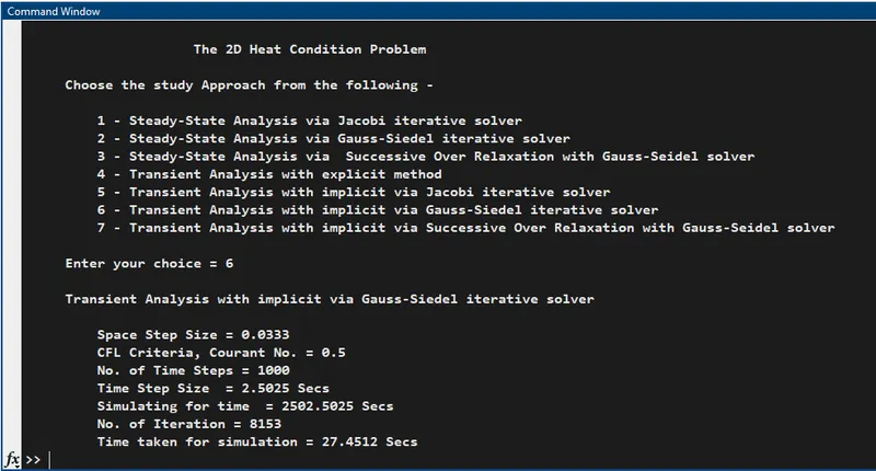
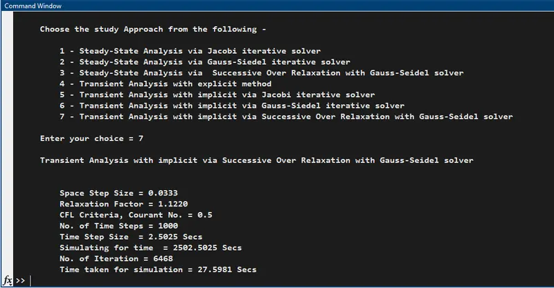
7. For Choice = 7, Transient Analysis with implicit via Successive Over Relaxation with Gauss-Seidel solver

RESULT -

• The following is the characteristics we observed for different solving methods -

Solving Approach	Iterations	Time Taken for Simulation (t)
Steady-State Analysis via Jacobi iterative solver	1896	0.3846 Seconds
Steady-State Analysis via Gauss-Siedel iterative solver	1016	0.5663 Seconds
Steady-State Analysis via Successive Over Relaxation with Gauss-Seidel solver	812	0.3117 Seconds
Transient Analysis with explicit method	--	25.9525 Seconds
Transient Analysis with implicit via Jacobi iterative solver	11567	26.5898 Seconds
Transient Analysis with implicit via Gauss-Siedel iterative solver	8153	27.4512 Seconds
Transient Analysis with implicit via Successive Over Relaxation with Gauss-Seidel solver	6468	27.5981 Seconds

• From the results we can compare the total iterations taken by the different approaches to converge the solution,

  For Steady-State solution, `I_((SOR)) < I_((GS)) < I_((Jacobi)) `

  For Transient-State solution, `I_(Implicit(SOR)) < I_(Implicit(GS)) < I_(Implicit(Jacobi)) `

  Hence, we see that in both Steady-state and transient analysis the the SOR method is the most effecient and fastest, taking least Iterations to converge the solution.But, it is also important to consider that the Steady-State Analysis does not include the Thermal Diffusivity and the time derivative terms therefore they are faster than the transient analysis.

  For the Explicit Method Iterations = 1000, thats nothing but the No. of timesteps itself. Explicit method doesn't require an Iterative solver it solves directly, it derives value of new time step by the values at the previous timestep. Therefore, the iterations or the no. of solving the stiffness matrix is limted to no. of time steps.

  A simulation analysis should be performed by keeping a perfect balance between Accuracy of the solution and the simulation time to solve it. Having a smaller time step will give is more precise and accurate results but may end up having larger simulation time.