MATLAB Program to simulate the motion Simple Pendulum as per the given data. (Matlab/Challenge-Week3-Solving second order ODEs)

Objective: Write a program in Matlab that simulate the motion Simple Pendulum with Damping. Use L = 1 metre, m = 1 kg, b = 0.05, g = 9.81 m/s2. Simulate the motion between time span of 0-20 sec, for angular displacement = 0, angular velocity=3 rad/sec at time t = 0.

Given data:

Length of the pendulum, L`=`1 metre

Mass of the Bob, m`=`1 kg

Damping Coefficient, b`=`0.05

Acceleration Gravity, g`=`9.81 m/s2

Angular Displacement (at time t=0), `theta =`0

Angular Velocity (at time t=0), `omega = (d theta)/(dt) =` 3 rad/sec

Time span = 0 - 20 sec

Theory:

A heavy body suspended by a light inextensible thread is called the simple pendulum. This is impracticable, so in practice, a small metal sphere is suspended from a rigid support using a cotton or silk thread. The point from which the bob is suspended is called point of suspension. The centre of gravity of the bob is called the centre of oscillations. The distance between the point of suspension and the centre of oscillations is called the length of the pendulum. The weight of the bob acts vertically downwards and the tension in the string acts vertically upwards. These two forces are equal and opposite and the bob has an equilibrium position in between.

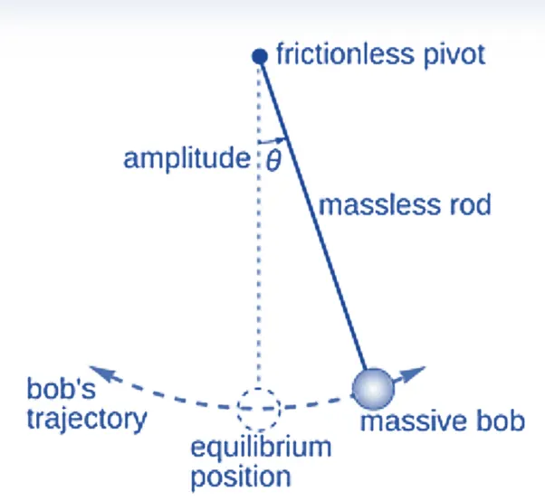
The motion of the simple pendulum is governed by the following ODE(Ordinary Differential Equation) -

`(d^2 theta)/dt^2 + (b/m)*(d theta)/dt +(g/l)*sintheta = 0`

Where, g = gravity in m/`s^2`

L = length of the pendulum in m

m = mass of the ball in kg

b = damping coefficient

Logic Used in Program:

The governing equation is the 2nd order differential equation, therefore to solve this equation in the program we simplify it to have the order of 1.

We consider, `theta_1 = theta` and so, `theta_2 = (d theta_1)/dt`

`=> (d theta_2)/dt = (d^2 theta_1)/dt^2`

`therefore` `(d theta_2)/dt + (b/m)*theta_2 +(g/l)*sintheta_1 = 0`

since, our required output here is `(d theta_2)/dt`

`=> (d theta_2)/dt = - (b/m*theta_2) -(g/l*sintheta_1)`

Program:

About the tool Used For the Problem -

ODE45 - it solves nonstiff differential equations — medium order method

Basic Syntax - [t, y] = ode45(odefun, tspan, y0)

where tspan = [t0 tf], integrates the system of differential equations y′=f(t, y) from t0 to tf with initial conditions y0. Each row in the solution array y corresponds to a value returned in column vector t.

In our case,

[t , r] = ode45(@(t, theta) ode_func(t, theta, b, l, g, m), t_span, theta0)

Where, @(t, theta) tells that the function ode_func is the function of t and theta. 't' is any time in the 'tspan' and 'theta' is position of the pendulum bob corresponding to time 't'.

1. Following is the program's Main function -

   % SIMULATING Pendulum and its Animation
   
   clear all
   close all
   clc
   b = 0.05;       % Damping coefficient
   l = 1;          % length od string of pendulum in 'm'      
   g = 9.81;       % Acceleration due to gravity in m/s^2
   m = 1;          % Mass of bob in 'kg'
   
   % Initial Condition
   theta_0 = [0; 3];
   
   % time points
   t_span = linspace(0,20,500);
   
   % Solving ODE 
   [t , results] = ode45(@(time, theta) pendulum_damped_ode_func(time, theta, b, l, g, m), t_span, theta_0);
   
   subplot(6,4,[17,18,21,22]);
   plot(t,results(:,1),'color','b','DisplayName','Position');
   hold on;
   plot(t,results(:,2), 'color','r','DisplayName','Angular Velocity');
   grid on;
   xlabel('Time (t)');
   ylabel('Position / Angular Velocity');
   title('Time vs Position/Angular Velocity');
   legend
   hold off;
   
   subplot(6,4,[19,20,23,24]);
   plot(results(:,1), results(:,2));
   grid on;
   xlabel('Position (Radians)');
   ylabel('Angular Velocity');
   title('Position vs Angular Velocity');
   
   ct = 1;             % ct is the counter variable.. here used for counting loop for getting frame
   
   for i = 1 : length(results(:,1))
       
       x0 = 0;     y0 = 0;
       x1 = l*sin(results(i,1));
       y1 = -l*cos(results(i,1));
       
       subplot(6,4,[1,2,3,4,5,6,7,8,9,10,11,12]);
       plot([-1 1],[0 0],'linewidth',3,'color','k');
       title('Pendulum Simulation');
       hold on
       line([x0 x1],[y0 y1],'linewidth',2,'color','b');
       
       
       r=0.25;
       rectangle('position',[(x1-r/2),(y1-r/2),r,r],'curvature',[1,1],'facecolor','r','linewidth',1.5);
       hold on;
       axis equal;
       
       % another way to make a circle -
       %r = 0.075;
       %cir_deg = linspace(0, 2*pi, 1000);
       %xc = r*cos(cir_deg);
       %yc = r*sin(cir_deg);
       %plot(x1+xc, y1+yc, 'linewidth', 2, 'color','r');
       %hold off;
       
       grid on;
       axis([-1.5 1.5 -1.5 0.5]);
       pause(0.1);                 % by pause command it pauses the code there for provided time 
       hold off;
       M(ct) = getframe(gcf);      % by getframe it Captures figure as movie frame
       ct = ct+1;
   end
   
   movie(M);                       % Play recorded movie frames
   video = VideoWriter('Pendulum_Dampped.avi','Uncompressed AVI'); 
   % Write video files and assigning video file name and video format
   open(video);            % Open file for writing video data
   writeVideo(video,M);    % Write video data to file
   close(video);           % Close file after writing video data
   

2. Following is a function which defines the Governing ODE -

   function [dtheta_dt] = pendulum_damped_ode_func(time, theta, b, l, g, m)
   
   theta1 = theta(1)
   theta2 = theta(2)
   
   dtheta1_dt = theta2;
   dtheta2_dt = - (b/m)*theta2 - (g/l)*sin(theta1);
   
   dtheta_dt = [dtheta1_dt; dtheta2_dt];
   
   end​

Output:

Simulation Video -

https://youtu.be/PYN2I86iV8I

https://drive.google.com/file/d/1jNIq4yuvETi3MH3dr5j0EzBlnBhlkisB/view?usp=sharing

Errors Faced -

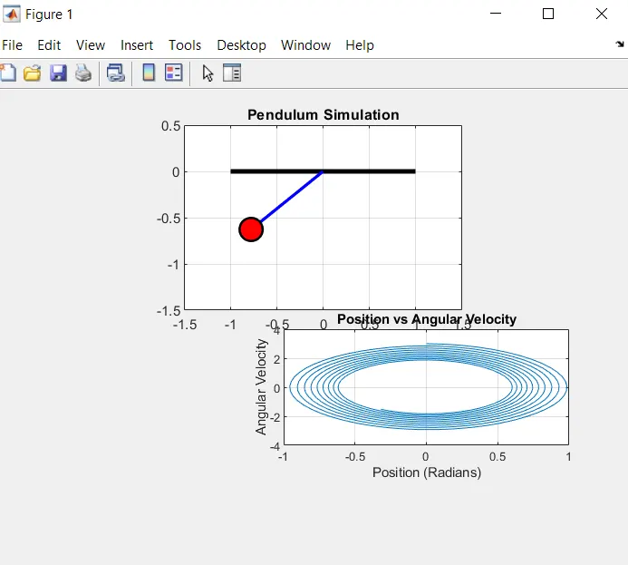
One of the problems was faced while using subplot. There were many problems, for examples overlapping of some elements. some missing plots due to mistake in allocation of plot.

It is shown in the screenshot below -