Week 11 - Louver/Grille characterization
AIM : To simulate the Hex Grille/louver geometry inorder get grille's loss coefficient via Parametrization method in Ansys Icepak.
OBJECTIVES :
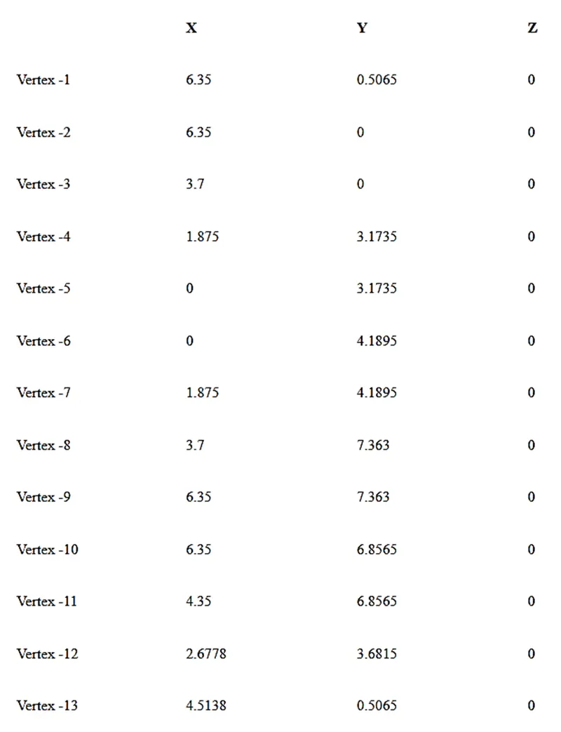
- Setting up the model Geometry via given polygon coordinate details.
- Create optimal meshing for the model using the bject mesh parameter.
- Setup the model for the Analysis.
- Run the simulation and Post Process the results.
INTRODUCTION :
Louvre/Grilles in electronic device is a ventilation for the device that allows air to pass through it whilst keeping out unwanted elements such as water, dirt and debris. They play a major role in electronic cooling of the device in both natural or forced convection cooling, as they are shield to the device but also an obstruction for the airflow from cabinet to ambient. It's also a factor for the access to volume of fresh(cool) air for cooling at a given time.
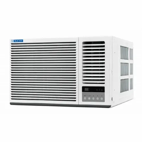
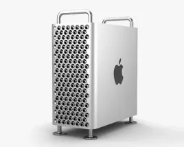
Simulations of electrical equipment, enclosed electronics components, and electrical systems are typical applications where grilles are used.The grille loss coefficient is a parameter whose value is a function not just of the free area ratio, but also of other parameters such as grille design, Reynolds number, grille thickness and flow regime (laminar or turbulent).
Icepak has an automatic mode that calculates the loss coefficient as a function of the free area ratio. However, this calculation is based on empirical correlations in the fully turbulent flow regime.Since most applications are for natural convection in the transitional flow regime it is important to develop a methodology to take into account the appropriate flow regime.
FOR HEX GRILLE -
1.1) Geometry
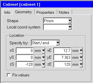
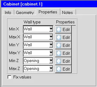
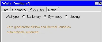
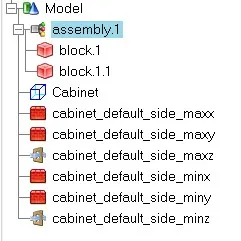
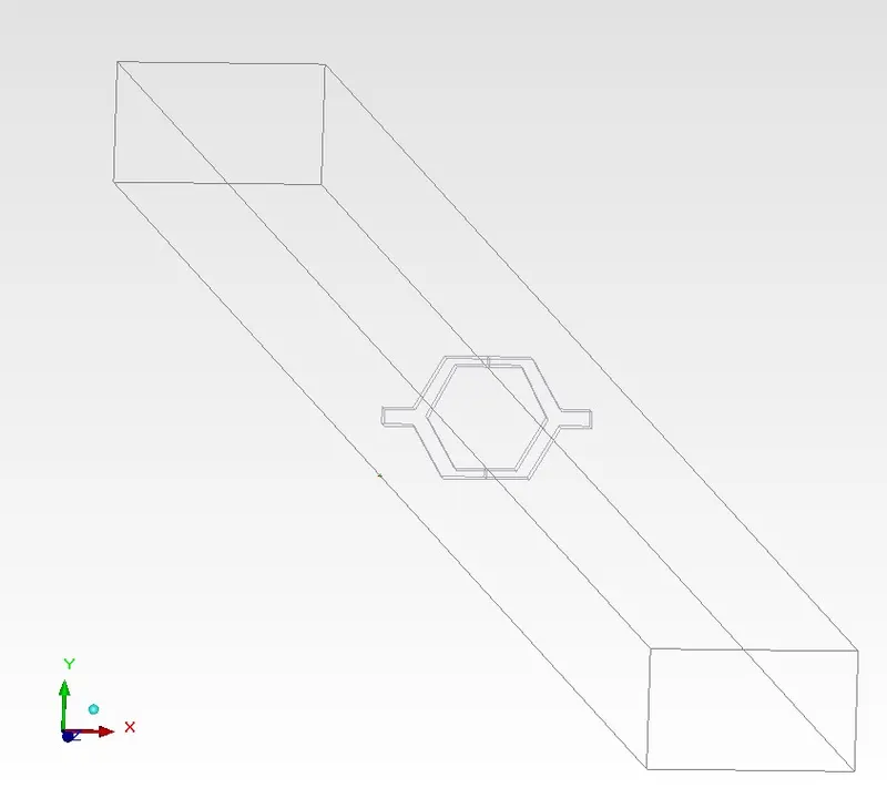
The model includes a cabinet that is 160 mm in length with inlet and outlet openings at the two ends (with a cross-sectional area of 7.363 mm x 12.7 mm), and four symmetry walls on the other sides. The model also includes a part of the Hexa-grille placed at the center of the channel in the streamwise direction, as shown in Figure.
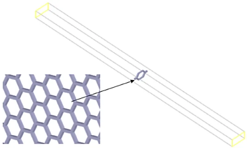
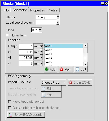
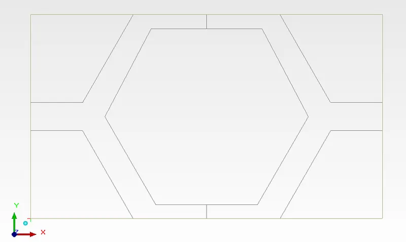
The grille has one full hexagonal hole at the center and four quarter hexagonal holes placed around it. This pattern was selected because it forms a periodic region and is sufficient to calculate the loss coefficient.
Following are the given coordinates for the Hex Grille geometry -
1.2) Meshing
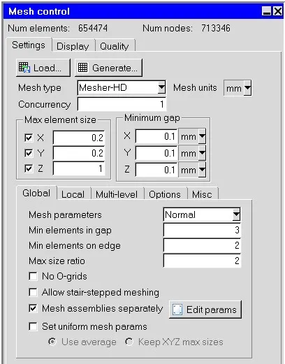
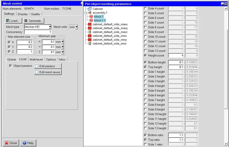
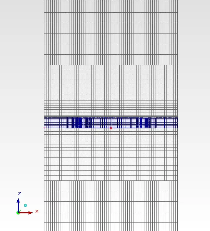
We have created a non-conformal mesh assembly accross the component assembly. To have fine mesh near to the components and coarser mesh across the enclosure and its ambient.
Following is setting used for global mesh and the assembly mesh settings -
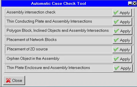
Case check tool in Macros options-

Mesh Quality Verification-
Following is the surface mesh of the Case Setup -
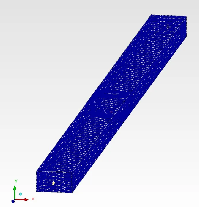
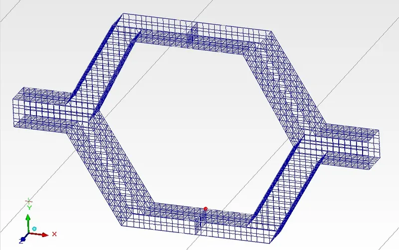
Following is the visualising the mesh inside the cabinet-
- Cut plane of XZ plane at 50% of the cabinet in Y-direction from origin (Top Plane)
Mesh Quality Parameters -
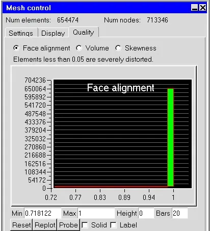
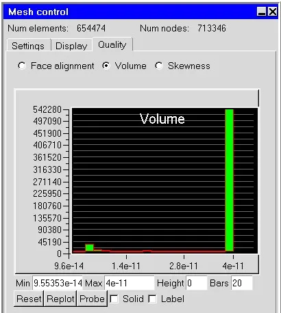
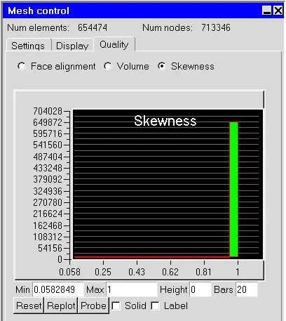
We can the mesh quality is very satisfied. 90% of the mesh cell are lying on good quality range.
1.3) Solver Settings -
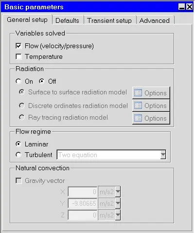
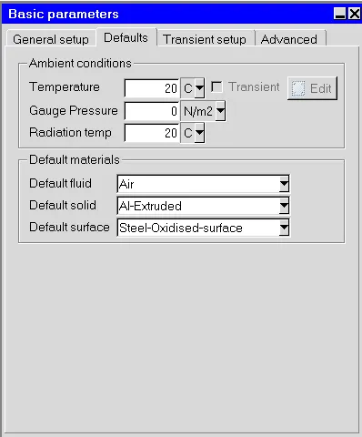
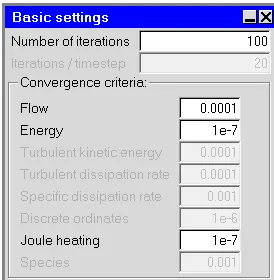
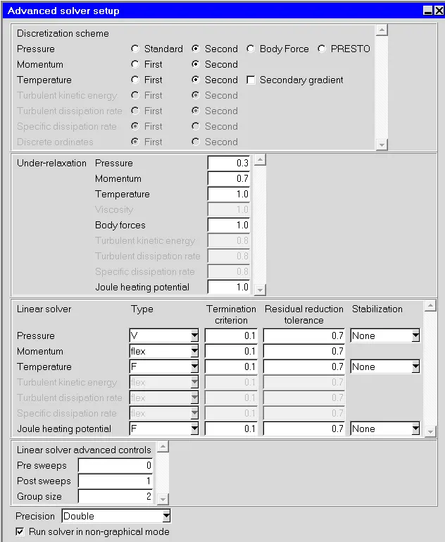
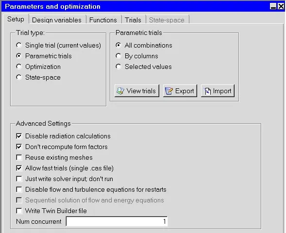
Assigning the values and settings for the Parametrization -
Calculation for the Parametrization with respect to reynold's no -
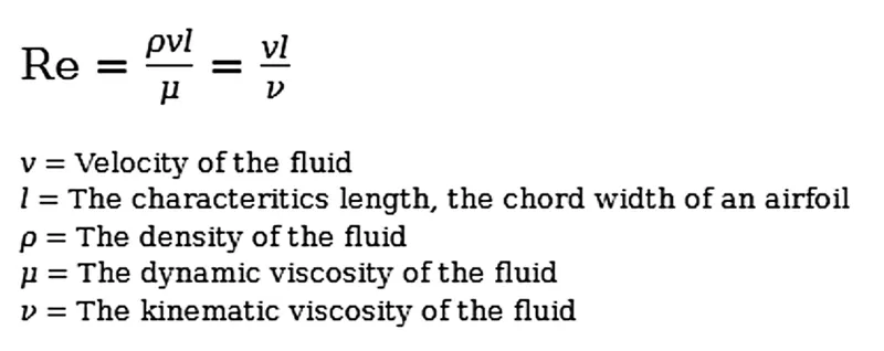
L or l = Characteristic length.
Here, `L = D_h = 4A/P`
`D_h = (4*(12.7*7.363)*1e^-6)/((2*12.7+2*7.363)*1e^-3)`
`D_h = 0.009321 m = 9.322e^-3 mm.`
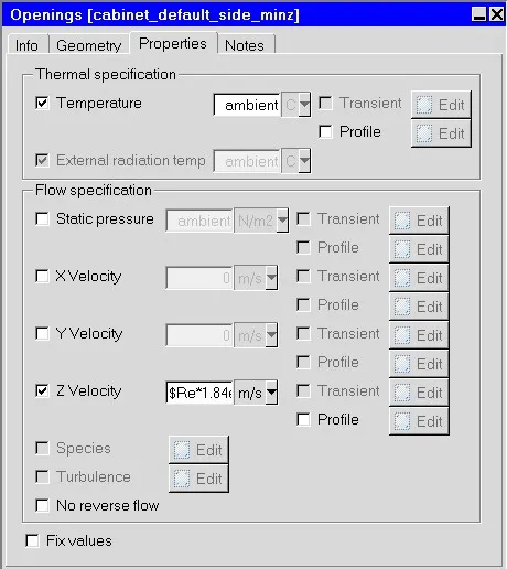
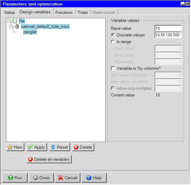
In Parameter and Optimization window,
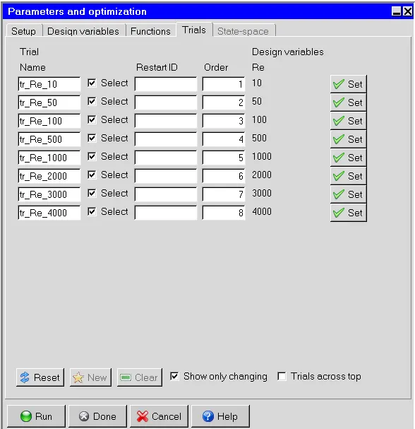
The parametric trails and the discrete values are set to 10 50 100 500 1000 2000 3000 4000.
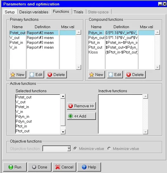
First we create primary functions,
i) Pstat_out - Cabinet_default_side_maxz_pressure (Mean)
ii) Vel_out - Cabinet_default_side_maxz_Uz (Mean)
iii) Pstat_in - Cabinet_default_side_minz_pressure (Mean)
iv) Vel_in - Cabinet_default_side_minz_pressure (Mean)
Now creating compound functions,
i) Pdyn_in - 0.5*1.16*$Vel_in*$Vel_in.
ii) Pdyn_out - 0.5*1.16*$Vel_out*$Vel_out.
iii) Ptot_in - $Pstat_in+$Pdyn_in.
iv) Ptot_out - $Pstat_out+$Pdyn_out.
v) Kloss - $Ptot_in - $Ptot_out / $Pdyn_out.
1.4) POST PROCESSING :
Outputs
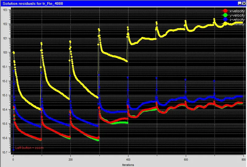
Residuals -
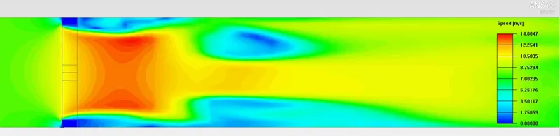
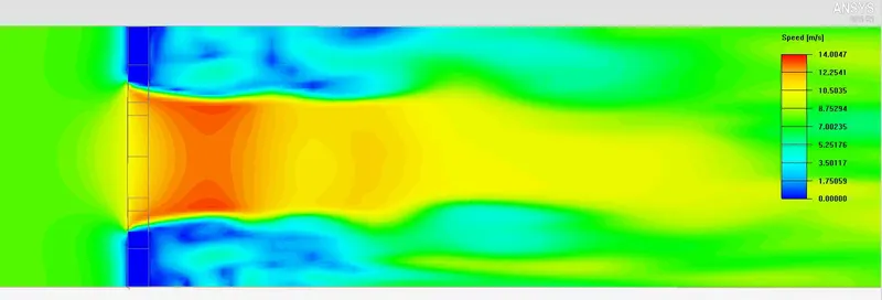
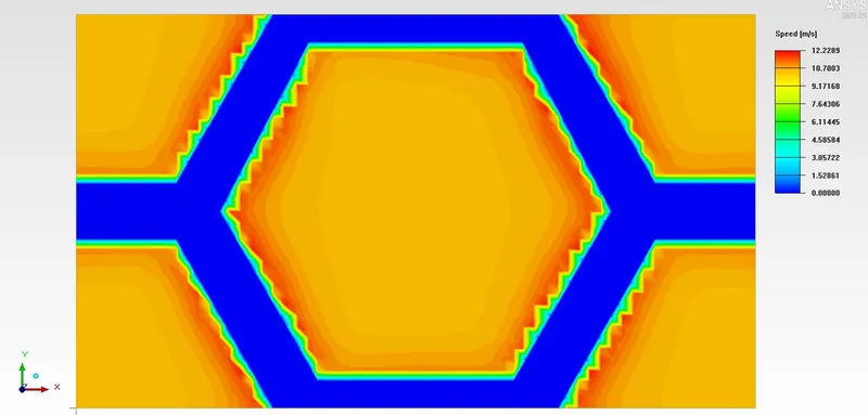
Velocity Contours -
Along X Direction-
Along Y Direction-
Along Z Direction at the Grille Cross-section -
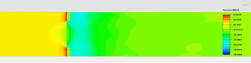
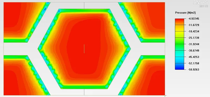
Pressure Contours -
Along Y Direction-
Along Z Direction at the Grille Cross-section -
1.5) RESULTS :
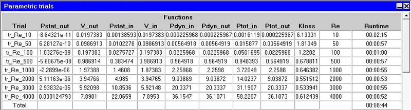
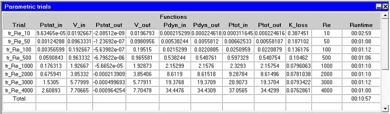
The Following are the Parametric results of the simulation, -
FOR LOUVER -
2.1) Geometry
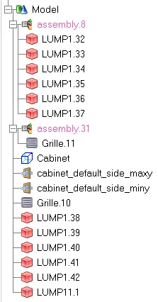
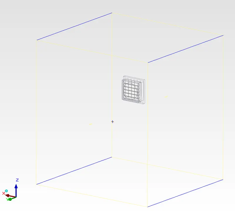
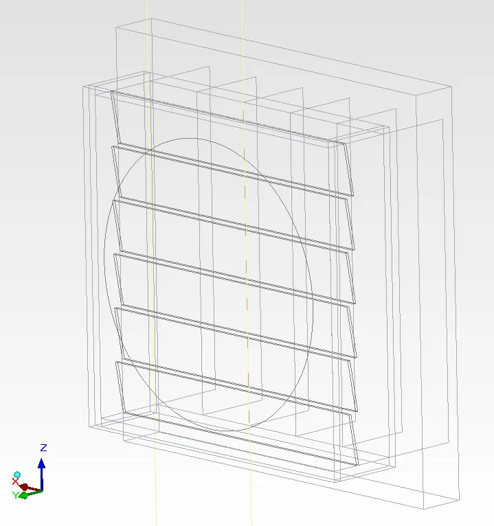
Unpacking the given project file and loading the given geometry for the louvers -
2.2) Meshing
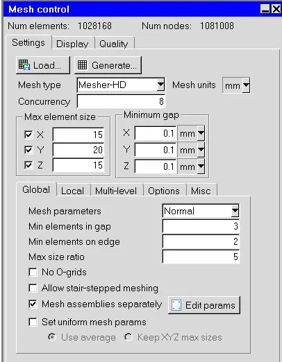
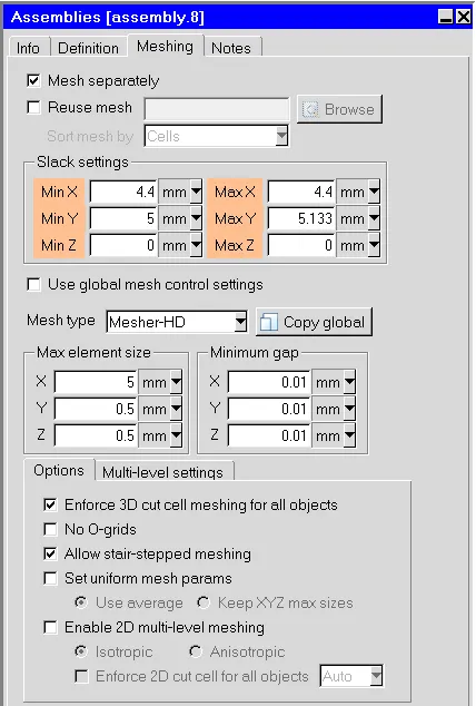
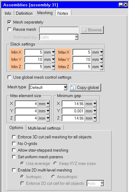
We have created a non-conformal mesh assembly accross the component assembly.
Following is mesh settings -
Case check tool in Macros options-
Mesh Quality Verification-
Following is the surface mesh of the Case Setup -
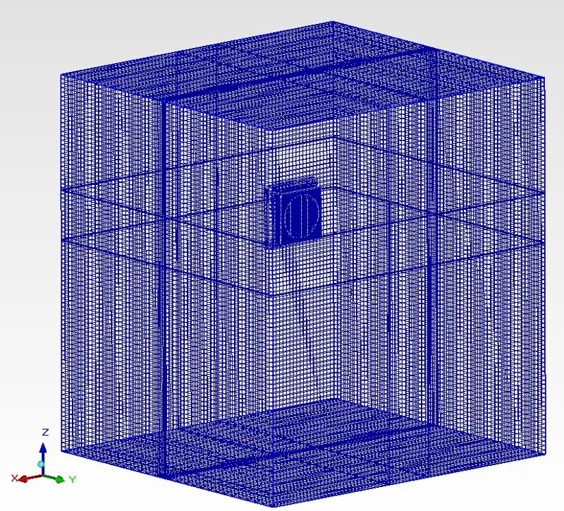
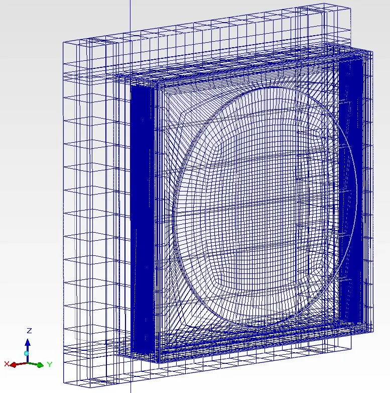
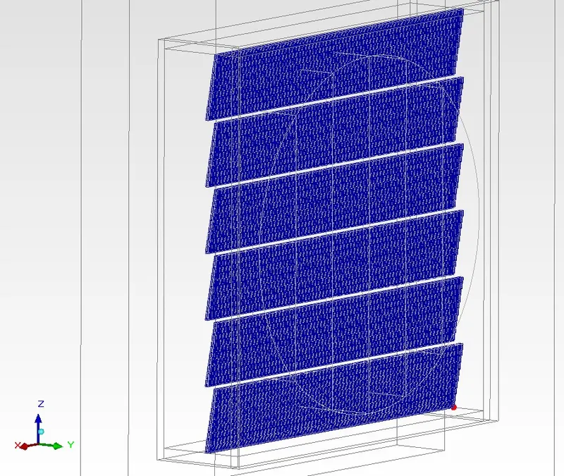
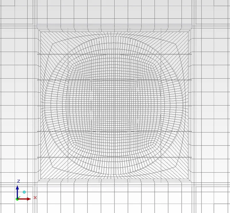
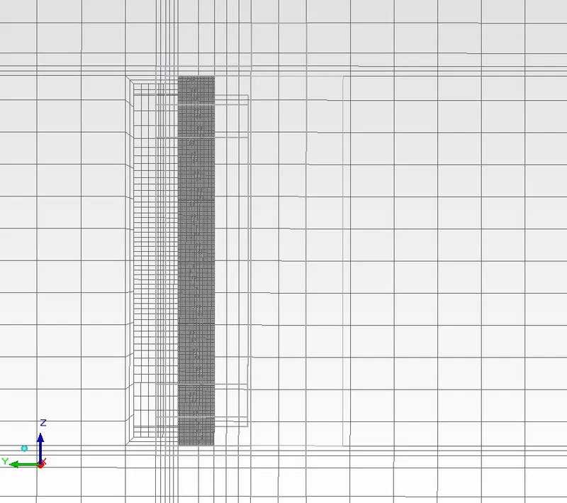
Following is the visualising the mesh inside the cabinet-
- Cut plane of XZ plane at 50% of the cabinet in Y-direction from origin (Front Plane)
- Cut plane of YZ plane at 50% of the cabinet in Y-direction from origin (Top Plane)
Mesh Quality Parameters -
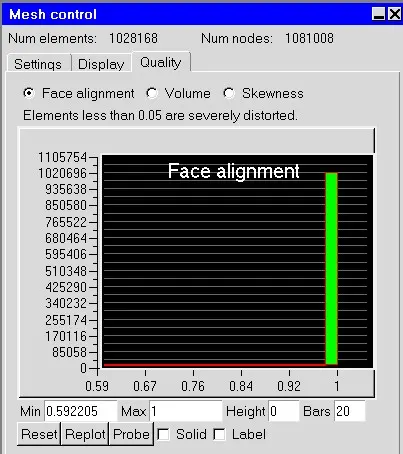
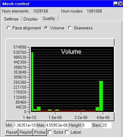
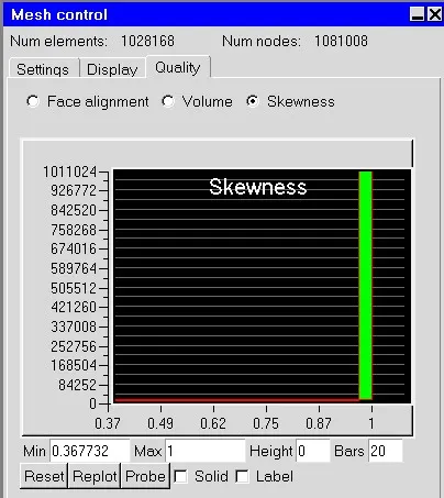
We can the mesh quality is very satisfied. 90% of the mesh cell are lying on good quality range.
2.3) Solver Settings -
Assigning the values and settings for the Parametrization -
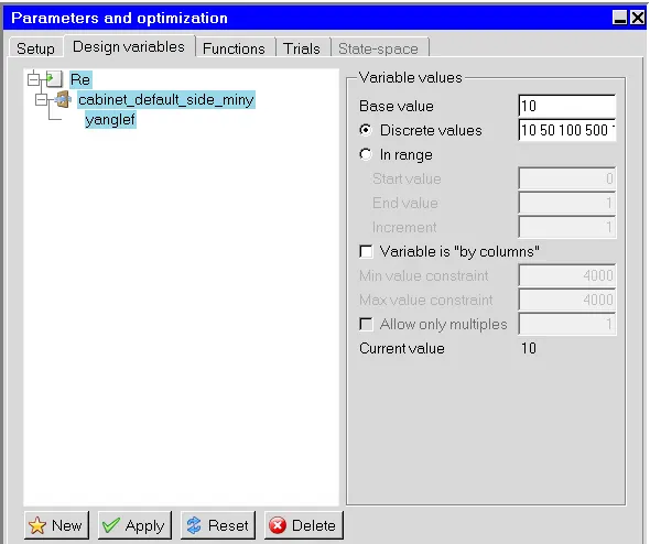
In Parameter and Optimization window,
The parametric trails and the discrete values are set to 10 50 100 500 1000 2000 3000 4000.
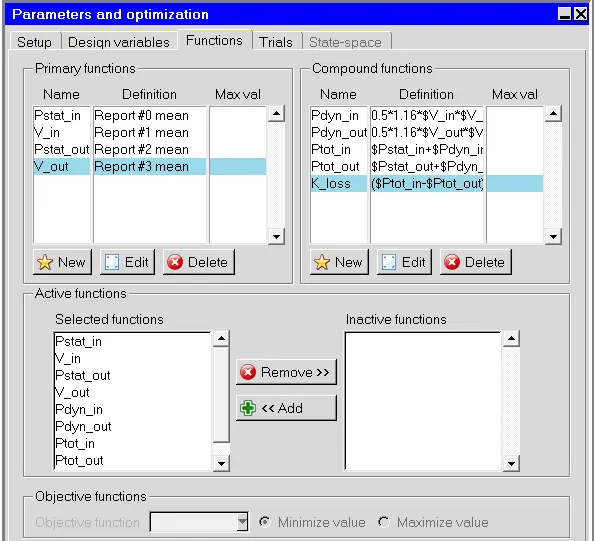
First we create primary functions,
i) Pstat_out - Cabinet_default_side_maxy_pressure (Mean)
ii) Vel_out - Cabinet_default_side_maxy_Uz (Mean)
iii) Pstat_in - Cabinet_default_side_miny_pressure (Mean)
iv) Vel_in - Cabinet_default_side_miny_pressure (Mean)
Now creating compound functions,
i) Pdyn_in - 0.5*1.16*$Vel_in*$Vel_in.
ii) Pdyn_out - 0.5*1.16*$Vel_out*$Vel_out.
iii) Ptot_in - $Pstat_in+$Pdyn_in.
iv) Ptot_out - $Pstat_out+$Pdyn_out.
v) Kloss - $Ptot_in - $Ptot_out / $Pdyn_out.
2.4) POST PROCESSING :
Outputs
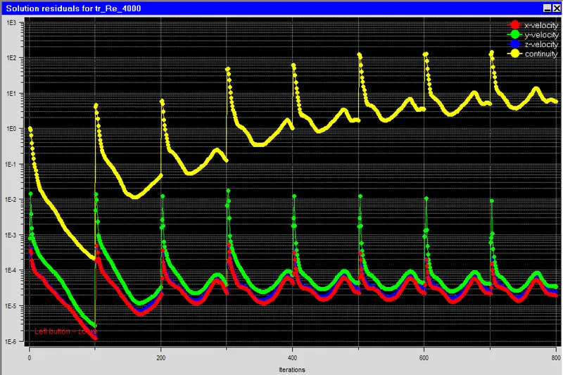
Residuals -
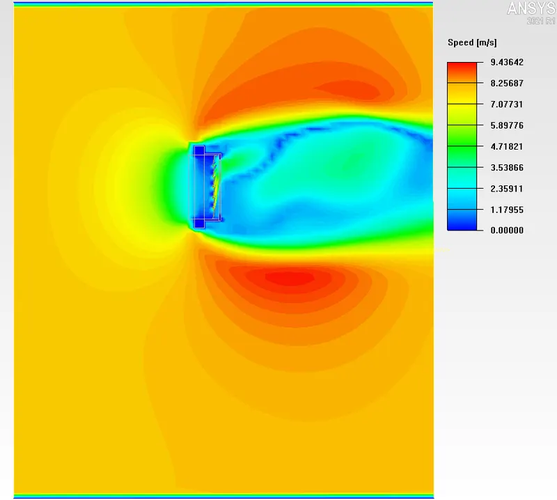
Velocity Contours -
Along X Direction-
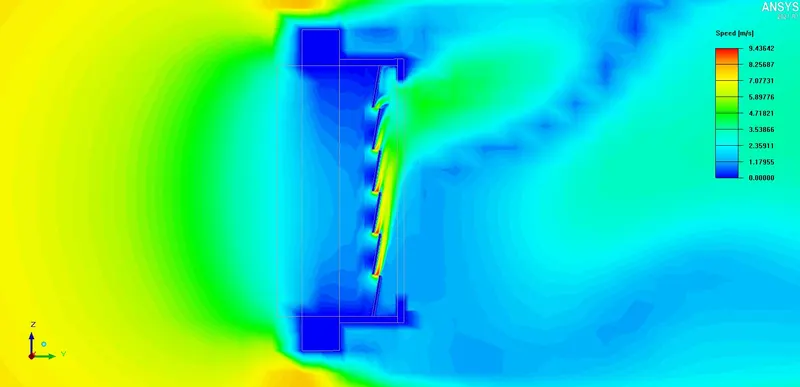
Along Z Direction at the Louver Cross-section -
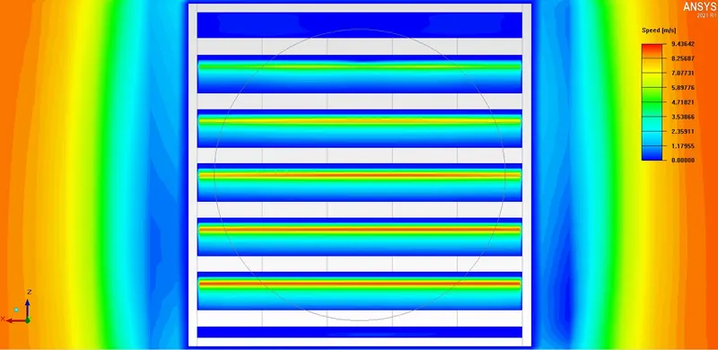
Pressure Contours -
Along X Direction-
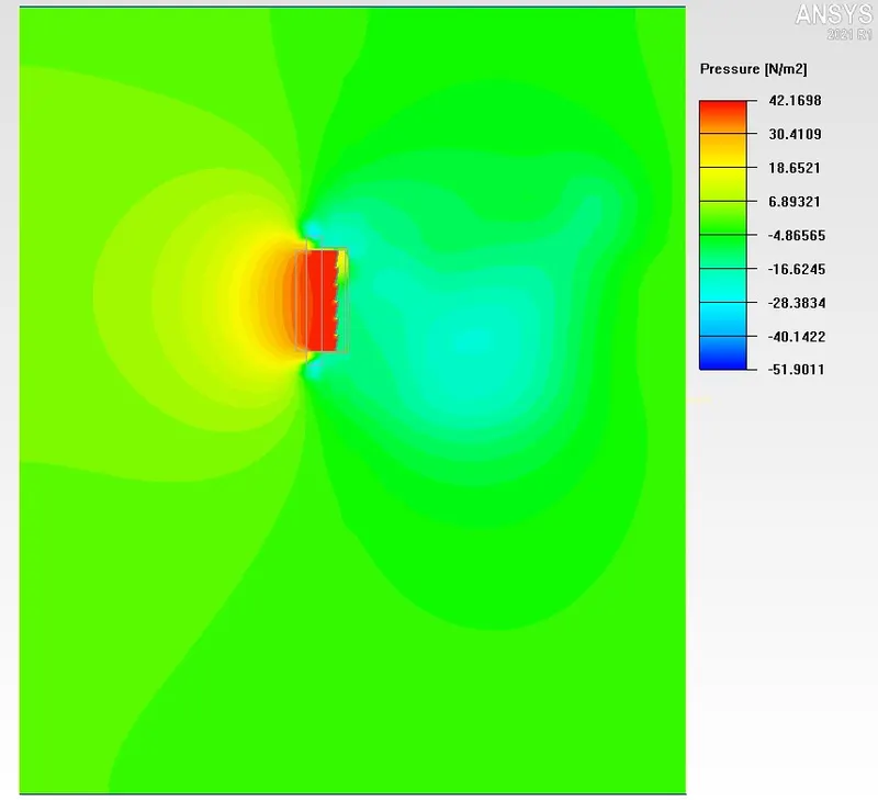
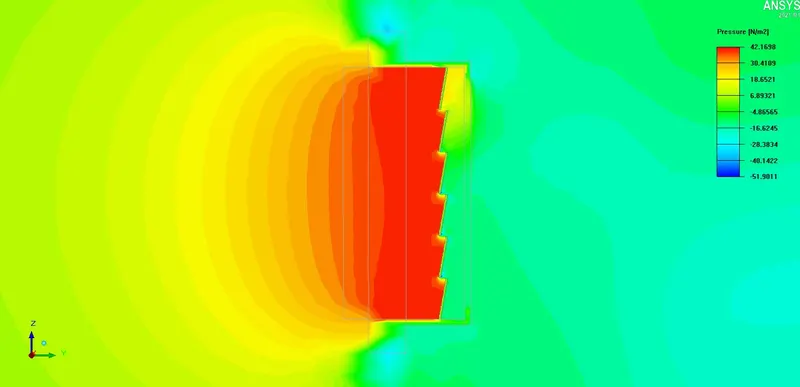
Along Z Direction at the Louver Cross-section -
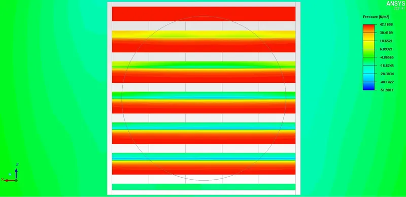
2.5) RESULTS :
The Following are the Parametric results of the simulation, -
CONCLUSION :
We have successfully performed the simulation analysis of the Forced Convection cooling via MRF approach.
In this challenge, we used the parameterization tool to calculate the loss coefficient of a grille for different values of Reynolds number (Re). We also defined other functions (e.g., static pressure and velocities at the inlet and outlet) that were reported for different Reynolds numbers. The results show that as Re increases, the loss coefficient decreases.
But we can the residuals were increasing with respect to the reynolds no., as the Re increases for more accuracy we can run for more no. of iteration. Also as the Re increases the requirement for more finer mesh respectively for more accuracy.
As conclusion, we can see how paraterization can be used for better analysis of the problem.