Simulation of Hagen-Poiseuille Flow through a pipe in OpenFOAM (ITCFDUML&OF/Challenge/Week-11)
AIM : Simulation of Flow through a Pipe (Hagen–Poiseuille Flow) in OpenFoam
OBJECTIVE :
- Write a program in Matlab that can generate the computational mesh automatically for any wedge angle.
- Select appropriate dimensions and condition for the problem
- Post process velocity profile, Pressure Drop and shear stress.
- Show that the velocity profile is fully developed.
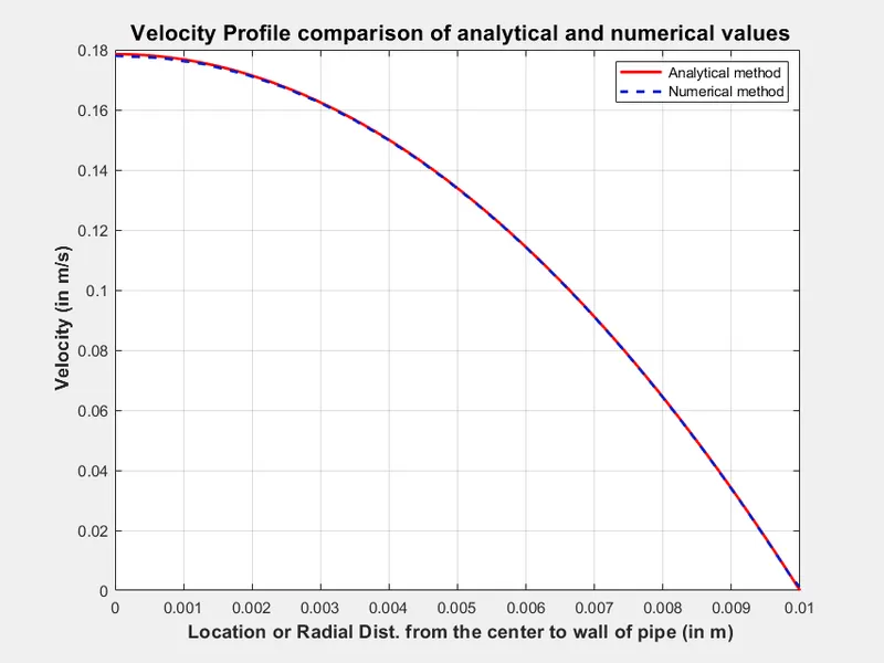
- Compare velocity profile calculated by numerical method with the velocity profile calculated with Hagen_poiseuille equation.
THEORY :
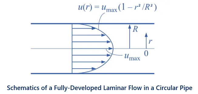
Hagen–Poiseuille Flow, is basically a fully-developed laminar flow in a pipe or duct . The mathematical model relationships for Pouiseuille flow relating the flow rate and/or velocity profile to the pressure drop along the pipe/duct, fluid viscosity and geometry are sometimes referred to as Poiseuille’s law (although strictly not a “law” of mechanics). The velocity profile of all Poiseuille flows is parabolic, and the rate of axial pressure drop is constant.
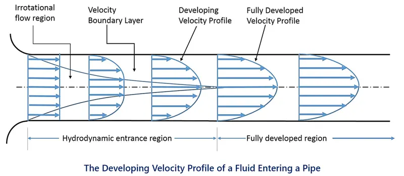
In the Laminar fluid flow inside a pipe, the surface contact between the water and the wall of the pipe will cause the water molecules to slow down and come to a complete stop near the walls. This layer of water molecules will also cause the adjacent layer of water flow to slow down due to the result of friction. To compensate for this velocity, water drops in the core of the pipe needs to maintain a constant velocity to keep the volumetric flow rate constant. As a result, the velocity boundary layer develops along the boundary walls of the pipe and starts to develop in the flow direction until it hits the center of the pipe. The distance from the pipe inlet to the point where the boundary layer merges is called the Hydrodynamic Entry Length. The region beyond the hydrodynamic entry length is known as the Fully Developed Region.
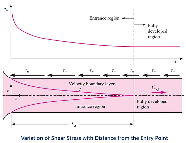
Shear stress (`tau_w`)
In the hydrodynamic entrance region, the wall shear stress (`tau_w`) is highest at the pipe inlet, where the boundary layer thickness is the smallest. Shear stress decreases along the flow direction.That is why the pressure drop is highest in the entrance region of a pipe, which increases the average friction factor for the whole pipe. This increase in the friction factor is negligible for long pipes.In a fully developed region, the pressure gradient and the shear stress in flow are in balance.
The Hagen-Poiseuille equation is a fluid mechanical equation that helps us understand how pressure varies in a flowing liquid. Specifically, it deals with pressure drops in viscous, Newtonian, incompressible fluids showing non-accelerated laminar flow (i.e. the flow is smooth).
`DeltaP = (8*mu*pi*L*Q)/(A^2) = (8*mu*L*V_(avg))/(R^2) = (32*mu*L*V_(avg))/(D^2)`
where,
`DeltaP` – Pressure Drop across the Pipe
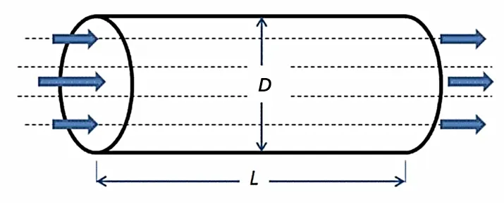
`D` – Diameter of the pipe , `R` – Radius of the pipe
`A` – C/S Area of the pipe
`mu` – Dynamic Viscosity of the fluid
L – Length of Pipe
`V_(avg)` – Average Velovity of the Fluid
`Q` – Volumetric Flow Rate of the Fluid
It has specific limitations, such as that it can be used only for long tubes that are cylindrical in shape, and with a uniform radius. Under these constraints, it is a really useful predictor of physical values.
PROBLEM CASE :
Considering a laminar fluid flow inside a pipe of diameter 'D', length 'L'. Taking the working fluid as water at temperature `25^@`C , and therefore the value of Density ( `rho` ) = 997 kg / `m^3` and Dynamic Viscosity ( `mu` ) = `8.90` x `10^-4` Pa.sec.
PARAMETERS & SETUP METHODLOGY :
Since the flow should be laminar and for the Flow through a Pipe the flow is laminar upto the Reynolds No. < 2300
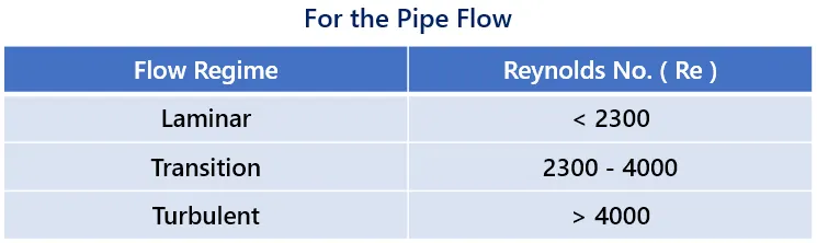
Therefore, selecting Reynolds No. for the flow to be Re = 2000.
Selecting the diameter of the pipe to be, D = 0.02
Now the Following formulas are used in order to calculate the important parameters, that satisfies the Hagen–Poiseuille Flow condition.
Hydrodynamic Entry length,
`L_E = 0.058*Re*D`
Average velocity,
`V_(avg) = (Re*mu)/(rho*D)`
Max Velocity,
`V_max = 2*Vavg`
Pressure difference,
`DeltaP = (32*mu*L*V_(avg))/D^2`
where,
`Re` – Reynolds Number, `mu` – Dynamic viscosity, `rho` – Density, `L` – Total Length of pipe,
Therefore,
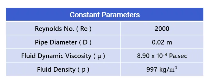
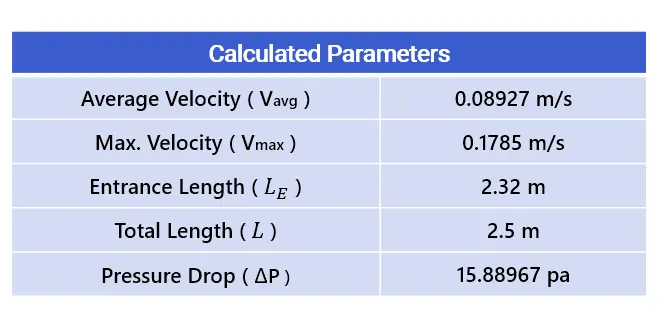
We know taht in a CFD simulation the significance of the mesh grid. The finer the grid more the resolution and more accurate the result. Inorder to capture near-wall physics where the fulid and body interacts we need more finer grid, this done by making the use of Grading/Inflation Layers technique in meshing. But more refined the grid is, more computational power and time it takes.
Therefore, inorder to reduces this comutation power and time while achieveing the main results, we can make use of Axis-Symmetric Nature of the flow problem. Here the Fluid is flowing through a cyclinderical pipe which axis-symmteric shape, and the fluid interaction and its resulting flow phenomenon happens in between from the wall to the center of the pipe.
Hence, we can reduced the computional domain as shown below -
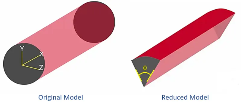
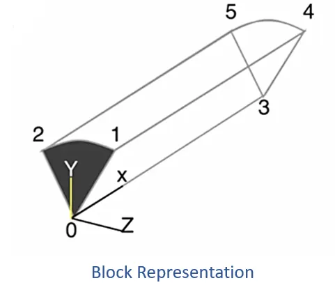
Now for the Reduced Model's C/S i.e. sector with angle `theta` . Taking the `theta = 4^@` for our simulation.
SIMULATION SETUP :
1. Choosing Solver Based on the Type of the Problem -
In this project case study, major physics the fluid flow problem accounts is laminar incompressible and viscous flow properties.
Therefore, for our problem, we will choose icoFoam solver in OpenFOAM i.e. basically incompressible solver, in which cavity problem is taken as base case in which, we gonna modify the files for geometry, boundary and initial conditions w.r.t to our problem.
Locating the tutorial problem similiar to our problem, which can solved by the same solver, and with slight modification in the setup.
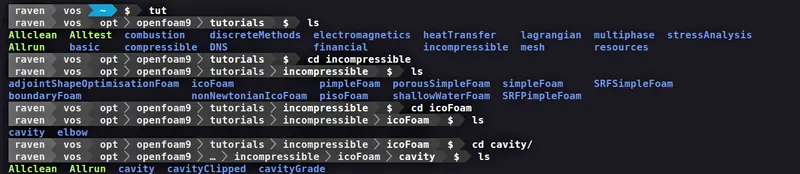
Now copy cavity folder from FOAM_TUTORIALS directory to the FOAM_RUN directory and rename it from the following command:
cp -r cavity/ $FOAM_RUN/pipeflow
2. Geometry and Meshing
The given Geometry and Dimensions of the geometry, is shown below -
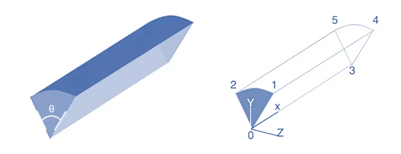
D = 0.02 m, R = 0.01 m, L =2.5 m, `theta = 4^@`
Meshing -
In OpenFOAM, the geometry and meshing parameters are defined in the blockMeshDict file. So inorder to define geometry for our problem we need to create the blockMeshDict file. For the current simulation problem we are gonna create a blockMeshDict File using MATLAB, with taking the reference of the existing blockMeshDict file from the tutorial case file we choosed.
MATLAB Program to create blockMeshDict File -
clear all
close all
clc

% Input parameters
    % Reynold's Number
    Re = 2000;
    % Total Length of pipe(m)
    L = 2.5;
    % Diameter of pipe in meters
    D = 0.02;
    % Wedge Angle in degrees
    theta = input('n Wedge/Sector Angle (in degrees) - ');
    % Density (kg/m^3)
    rho = 997;
    % Dynamic Viscosity (Pa.sec)
    mu = 8.90e-4;
    % Radius of pipe(m)
    R = D/2;


% Entrance Length
Le = 0.058*Re*D;

% Number of cells in x,y,z Directions
nx = 500;
ny = 30;
nz = 1;

%------------------------------------------------------------------------
%        BlockMeshDict file writting
%------------------------------------------------------------------------

f1 = fopen('blockMeshDict','w');

    fprintf(f1,'%s n','/*--------------------------------*- C++ -*----------------------------------*');
    fprintf(f1,'%s n','  =========                 |');
    fprintf(f1,'%s n','        /  F ield         | OpenFOAM: The Open Source CFD Toolbox');
    fprintf(f1,'%s n','       /   O peration     | Website:  https://openfoam.org');
    fprintf(f1,'%s n','      /    A nd           | Version:  9');
    fprintf(f1,'%s n','     /     M anipulation  |');
    fprintf(f1,'%s n','*---------------------------------------------------------------------------*/');
    fprintf(f1,'FoamFile n');
    fprintf(f1,'{ n');
    fprintf(f1,'    format      ascii;n');
    fprintf(f1,'    class       dictionary;n');
    fprintf(f1,'    object      blockMeshDict;n');
    fprintf(f1,'} n');
    fprintf(f1,'%s nn','// * * * * * * * * * * * * * * * * * * * * * * * * * * * * * * * * * * * * * // ');
    fprintf(f1,'convertToMeters 1; nn');
    fprintf(f1,'verticesn( n');
    fprintf(f1, '   /* 0 */ (0 0 0) n');
    fprintf(f1,('   /* 1 */ (0 %f %f) n'),R*cosd(theta/2),R*sind(theta/2));
    fprintf(f1,('   /* 2 */ (0 %f %f)n'),R*cosd(theta/2),-R*sind(theta/2));
    fprintf(f1,('   /* 3 */ (%f 0 0)n'),L);
    fprintf(f1,('   /* 4 */ (%f %f %f)n'),L,R*cosd(theta/2),R*sind(theta/2));
    fprintf(f1,('   /* 5 */ (%f %f %f)n);nn'),L,R*cosd(theta/2),-R*sind(theta/2));
    fprintf(f1,'blocksn(n');
    fprintf(f1,('hex (0 2 1 0 3 5 4 3) (%d %d %d) simpleGrading (0.2 1 1)n);nn'),ny,nz,nx);
    fprintf(f1,'edgesn(n');
    fprintf(f1,'    arc 2 1 (0 %f 0)n',R);
    fprintf(f1,'    arc 5 4 (%f %f 0)n);nn',L,R);
    fprintf(f1,'boundaryn(n');
    fprintf(f1,'     inletn');
    fprintf(f1,'     {n');
    fprintf(f1,'           type patch;n');
    fprintf(f1,'           facesn');
    fprintf(f1,'           (n');
    fprintf(f1,'               (0 1 2 0)n');
    fprintf(f1,'           );n');
    fprintf(f1,'     }n');
    fprintf(f1,'     outletn');
    fprintf(f1,'     {n');
    fprintf(f1,'           type patch;n');
    fprintf(f1,'           facesn');
    fprintf(f1,'           (n');
    fprintf(f1,'               (3 5 4 3)n');
    fprintf(f1,'           );n');
    fprintf(f1,'     }n');
    fprintf(f1,'     frontn');
    fprintf(f1,'     {n');
    fprintf(f1,'           type wedge;n');
    fprintf(f1,'           facesn');
    fprintf(f1,'           (n');
    fprintf(f1,'               (0 3 4 1)n');
    fprintf(f1,'           );n');
    fprintf(f1,'     }n');
    fprintf(f1,'     backn');
    fprintf(f1,'     {n');
    fprintf(f1,'           type wedge;n');
    fprintf(f1,'           faces n');
    fprintf(f1,'           (n');
    fprintf(f1,'               (0 2 5 3)n');
    fprintf(f1,'           );n');
    fprintf(f1,'     }n');
    fprintf(f1,'     pipewalln');
    fprintf(f1,'     {n');
    fprintf(f1,'           type wall;n');
    fprintf(f1,'           facesn');
    fprintf(f1,'           (n');
    fprintf(f1,'               (1 4 5 2)n');
    fprintf(f1,'           );n');
    fprintf(f1,'     }n');
    fprintf(f1,'     axisn');
    fprintf(f1,'     {n');
    fprintf(f1,'           type empty;n');
    fprintf(f1,'           facesn');
    fprintf(f1,'           (n');
    fprintf(f1,'               (0 3 3 0)n');
    fprintf(f1,'           );n');
    fprintf(f1,'      }n');
    fprintf(f1,');nn');
    fprintf(f1,'mergePatchPairsn');
    fprintf(f1,'(n');
    fprintf(f1,');nn');
    fprintf(f1,'// ************************************************************************* // n');

fclose(f1);
blockMeshDict File -
/*--------------------------------*- C++ -*----------------------------------*
  =========                 |
        /  F ield         | OpenFOAM: The Open Source CFD Toolbox
       /   O peration     | Website:  https://openfoam.org
      /    A nd           | Version:  9
     /     M anipulation  |
*---------------------------------------------------------------------------*/
FoamFile
{
    format      ascii;
    class       dictionary;
    object      blockMeshDict;
}
// * * * * * * * * * * * * * * * * * * * * * * * * * * * * * * * * * * * * * //

convertToMeters 1;

vertices
(
   /* 0 */ (0 0 0)
   /* 1 */ (0 0.009994 0.000349)
   /* 2 */ (0 0.009994 -0.000349)
   /* 3 */ (2.500000 0 0)
   /* 4 */ (2.500000 0.009994 0.000349)
   /* 5 */ (2.500000 0.009994 -0.000349)
);

blocks
(
hex (0 2 1 0 3 5 4 3) (30 1 500) simpleGrading (0.2 1 1)
);

edges
(
    arc 2 1 (0 0.010000 0)
    arc 5 4 (2.500000 0.010000 0)
);

boundary
(
     inlet
     {
           type patch;
           faces
           (
               (0 1 2 0)
           );
     }
     outlet
     {
           type patch;
           faces
           (
               (3 5 4 3)
           );
     }
     front
     {
           type wedge;
           faces
           (
               (0 3 4 1)
           );
     }
     back
     {
           type wedge;
           faces
           (
               (0 2 5 3)
           );
     }
     pipewall
     {
           type wall;
           faces
           (
               (1 4 5 2)
           );
     }
     axis
     {
           type empty;
           faces
           (
               (0 3 3 0)
           );
      }
);

mergePatchPairs
(
);

// ************************************************************************* //
3. Simulation Run Setup -
controlDict File -
/*--------------------------------*- C++ -*----------------------------------*
  =========                 |
        /  F ield         | OpenFOAM: The Open Source CFD Toolbox
       /   O peration     | Website:  https://openfoam.org
      /    A nd           | Version:  9
     /     M anipulation  |
*---------------------------------------------------------------------------*/
FoamFile
{
    format      ascii;
    class       dictionary;
    location    "system";
    object      controlDict;
}
// * * * * * * * * * * * * * * * * * * * * * * * * * * * * * * * * * * * * * //

application     icoFoam;

startFrom       startTime;

startTime       0;

stopAt          endTime;

endTime         0.5;

deltaT          0.0002;

writeControl    timeStep;

writeInterval   5;

purgeWrite      0;

writeFormat     ascii;

writePrecision  6;

writeCompression off;

timeFormat      general;

timePrecision   6;

runTimeModifiable true;


// ************************************************************************* //
4. Initial and Boundary Conditions -
P -
/*--------------------------------*- C++ -*----------------------------------*
  =========                 |
        /  F ield         | OpenFOAM: The Open Source CFD Toolbox
       /   O peration     | Website:  https://openfoam.org
      /    A nd           | Version:  9
     /     M anipulation  |
*---------------------------------------------------------------------------*/
FoamFile
{
    format      ascii;
    class       volScalarField;
    object      p;
}
// * * * * * * * * * * * * * * * * * * * * * * * * * * * * * * * * * * * * * //

dimensions      [0 2 -2 0 0 0 0];

internalField   uniform 0;

boundaryField
{
    inlet
    {
        type            zeroGradient;
    }

    outlet
    {
        type            fixedValue;
        value           uniform 0;
    }

    front
    {
        type            wedge;
    }

    back
    {
        type            wedge;
    }

    axis
    {
        type            empty;
    }

    pipewall
    {
        type            zeroGradient;
    }
}

// ************************************************************************* //
U -
/*--------------------------------*- C++ -*----------------------------------*
  =========                 |
        /  F ield         | OpenFOAM: The Open Source CFD Toolbox
       /   O peration     | Website:  https://openfoam.org
      /    A nd           | Version:  9
     /     M anipulation  |
*---------------------------------------------------------------------------*/
FoamFile
{
    format      ascii;
    class       volVectorField;
    object      U;
}
// * * * * * * * * * * * * * * * * * * * * * * * * * * * * * * * * * * * * * //

dimensions      [0 1 -1 0 0 0 0];

internalField   uniform (0 0 0);

boundaryField
{
    inlet
    {
        type            fixedValue;
        value           uniform (0.08927 0 0);
    }

    outlet
    {
        type            zeroGradient;
    }

    front
    {
        type            wedge;
    }

    back
    {
        type            wedge;
    }

    axis
    {
        type            empty;
    }

    pipewall
    {
        type            noSlip;
    }
}

// ************************************************************************* //
transportProperties File -
/*--------------------------------*- C++ -*----------------------------------*
  =========                 |
        /  F ield         | OpenFOAM: The Open Source CFD Toolbox
       /   O peration     | Website:  https://openfoam.org
      /    A nd           | Version:  9
     /     M anipulation  |
*---------------------------------------------------------------------------*/
FoamFile
{
    format      ascii;
    class       dictionary;
    location    "constant";
    object      transportProperties;
}
// * * * * * * * * * * * * * * * * * * * * * * * * * * * * * * * * * * * * * //

nu              [0 2 -1 0 0 0 0] 8.90e-4;


// ************************************************************************* //
FVSchemes & FVSolution :
Along with the blockMeshDict and controlDict files there are also fvschemes and fvSolution files in the system folder.
fvSchemes script file sets the numerical schemes for terms, such as derivatives in equations, that are calculated during a simulation.
fvSchemes -
/*--------------------------------*- C++ -*----------------------------------*
  =========                 |
        /  F ield         | OpenFOAM: The Open Source CFD Toolbox
       /   O peration     | Website:  https://openfoam.org
      /    A nd           | Version:  9
     /     M anipulation  |
*---------------------------------------------------------------------------*/
FoamFile
{
    format      ascii;
    class       dictionary;
    location    "system";
    object      fvSchemes;
}
// * * * * * * * * * * * * * * * * * * * * * * * * * * * * * * * * * * * * * //

ddtSchemes
{
    default         Euler;
}

gradSchemes
{
    default         Gauss linear;
    grad(p)         Gauss linear;
}

divSchemes
{
    default         none;
    div(phi,U)      Gauss linear;
}

laplacianSchemes
{
    default         Gauss linear orthogonal;
}

interpolationSchemes
{
    default         linear;
}

snGradSchemes
{
    default         orthogonal;
}


// ************************************************************************* //
The equation solvers, tolerances and algorithms are controlled from the fvSolution dictionary in the system directory. Below in our problem, set of entries from the fvSolution dictionary required for the icoFoam solver.
fvSolution -
/*--------------------------------*- C++ -*----------------------------------*
  =========                 |
        /  F ield         | OpenFOAM: The Open Source CFD Toolbox
       /   O peration     | Website:  https://openfoam.org
      /    A nd           | Version:  9
     /     M anipulation  |
*---------------------------------------------------------------------------*/
FoamFile
{
    format      ascii;
    class       dictionary;
    location    "system";
    object      fvSolution;
}
// * * * * * * * * * * * * * * * * * * * * * * * * * * * * * * * * * * * * * //

solvers
{
    p
    {
        solver          PCG;
        preconditioner  DIC;
        tolerance       1e-06;
        relTol          0.05;
    }

    pFinal
    {
        $p;
        relTol          0;
    }

    U
    {
        solver          smoothSolver;
        smoother        symGaussSeidel;
        tolerance       1e-05;
        relTol          0;
    }
}

PISO
{
    nCorrectors     2;
    nNonOrthogonalCorrectors 0;
    pRefCell        0;
    pRefValue       0;
}


// ************************************************************************* //
POST-POSTPROCESSING & RESULTS -
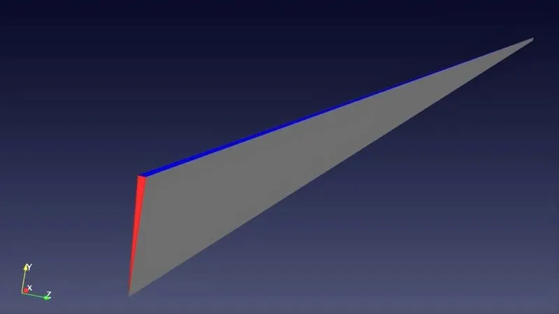
1. Geometry & Mesh Generated -
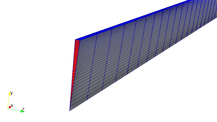
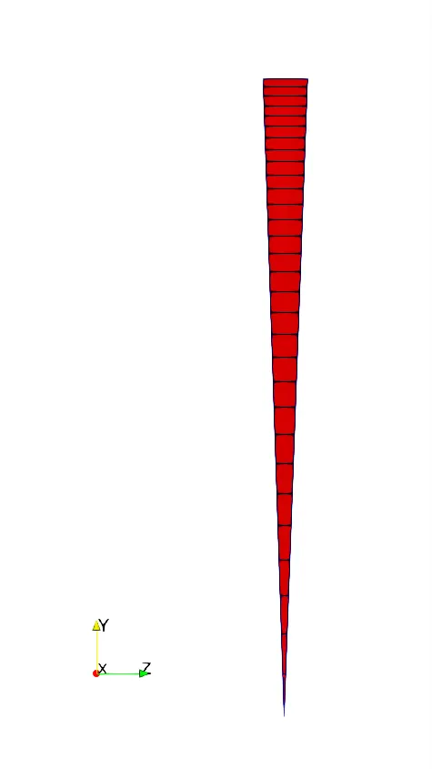
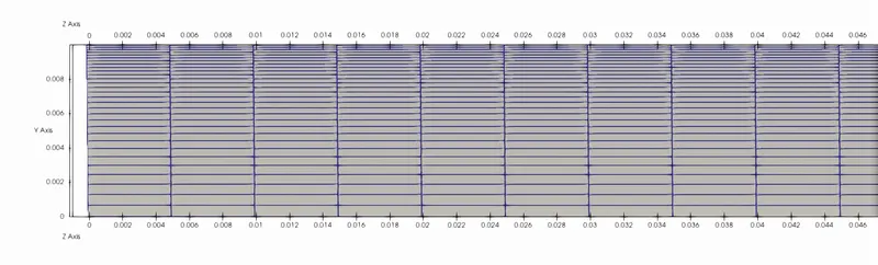
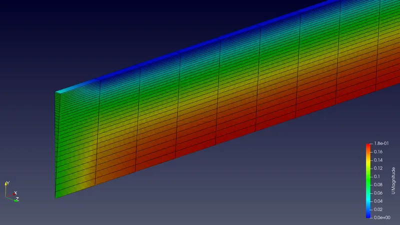
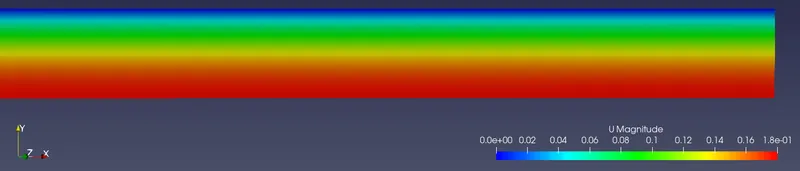
2. Velocity Contour -
At inlet -
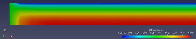
At Outlet -
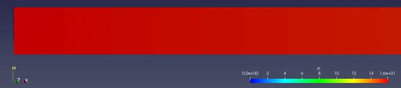
3. Pressure Contour -
At inlet -
At Outlet -
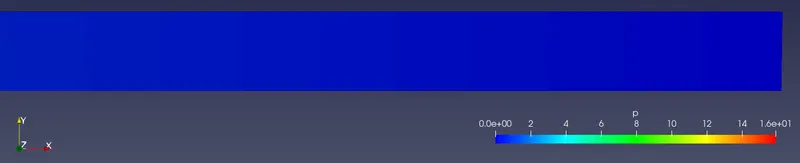
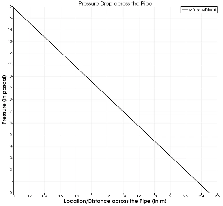
4. Pressure Drop Across the Pipe -

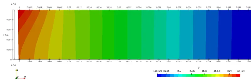
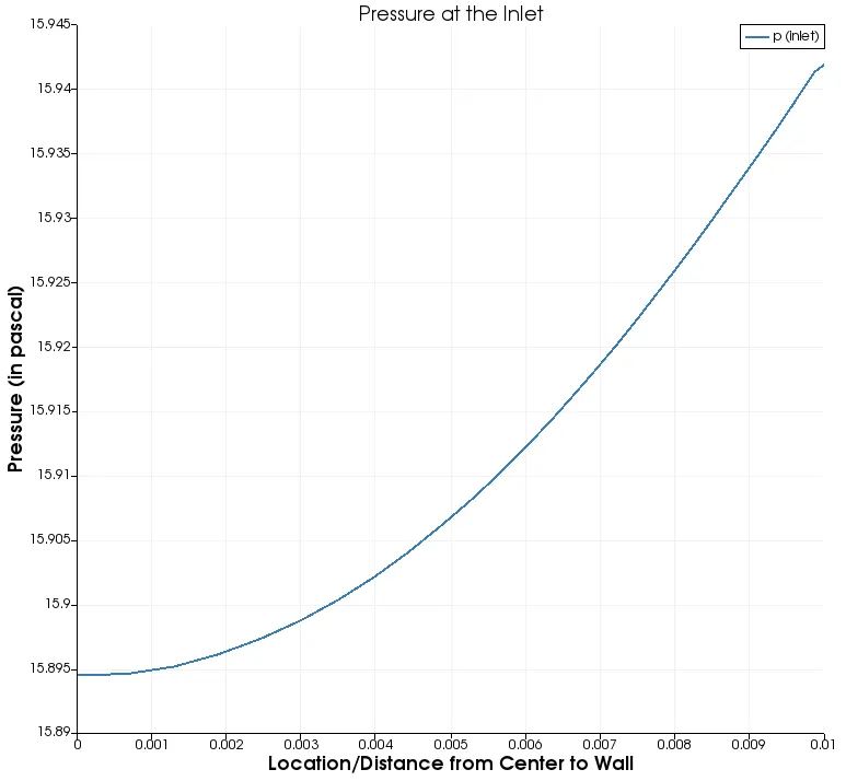
4. Pressure Profile at the Inlet of the Pipe
Pressure contour (with Local Legend Range) -
Pressure Profile at the Inlet wall -
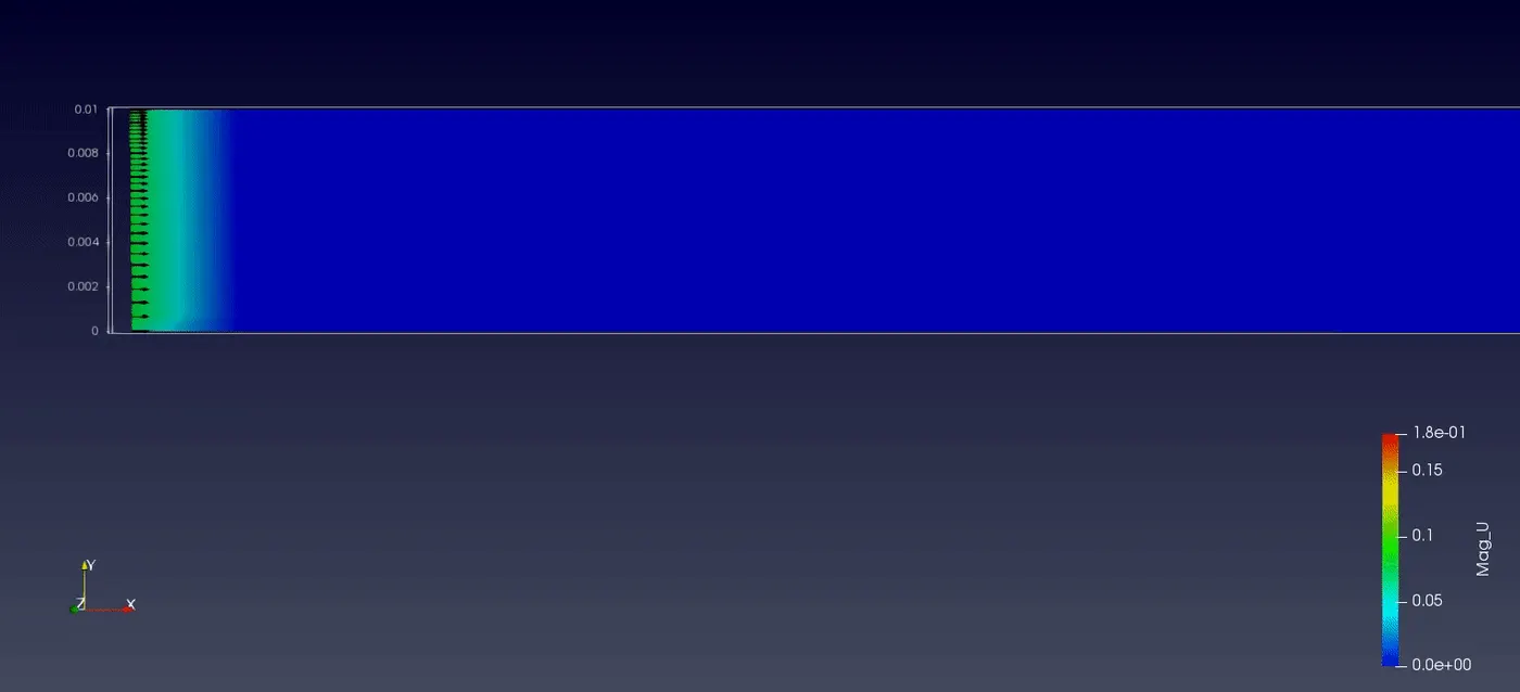
5. Velocity Profiles :
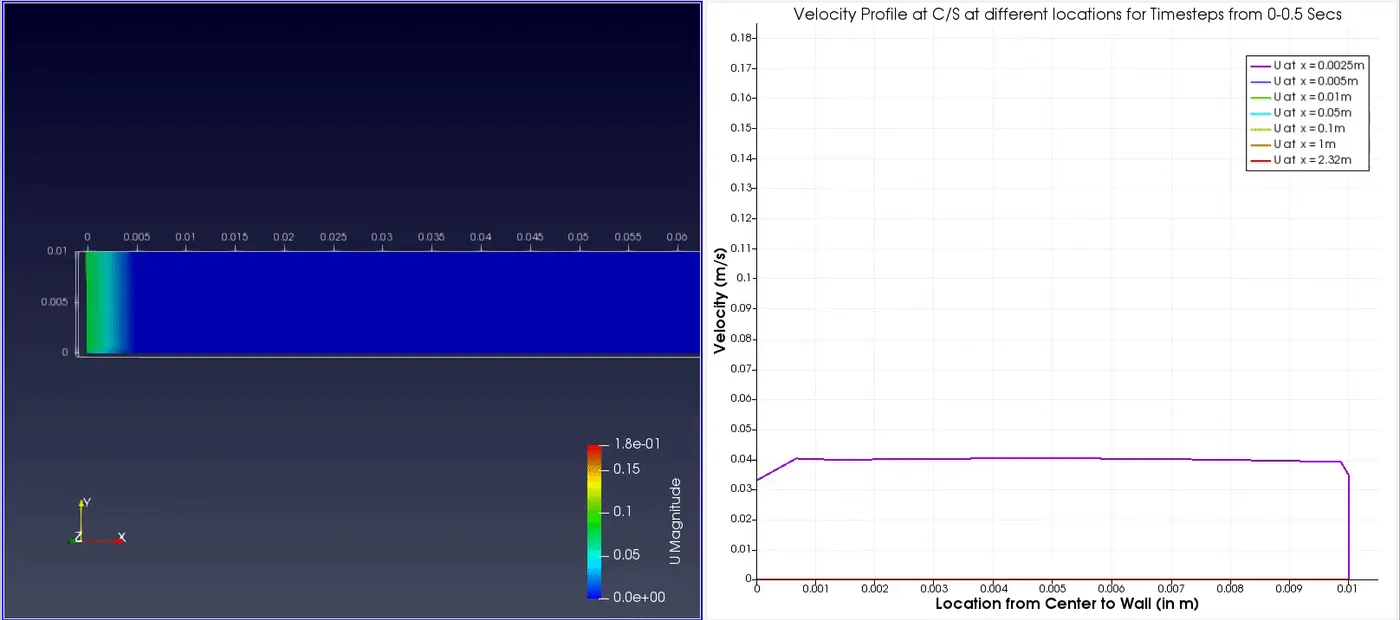
Velocity Profiles near the Inlet Entry w.r.t time from 0 to 0.5 secs -
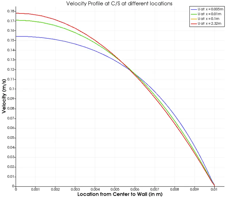
Velocity Profile Developement and Comparison at different locations across the pipe w.r.t to time 0-0.5 secs -
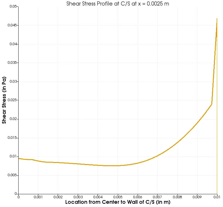
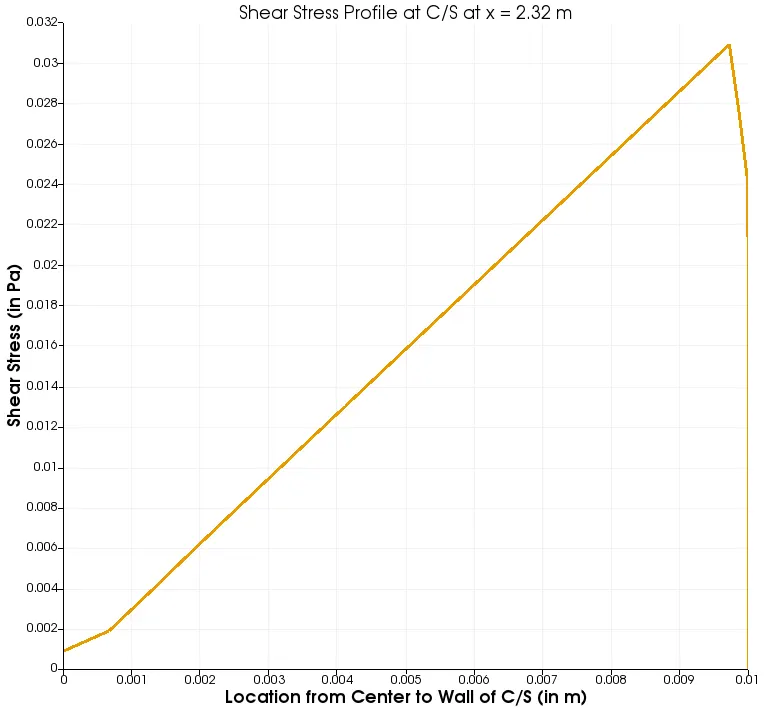
6. Shear Stress Profile -
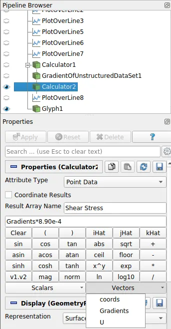
Now for estimating the Shear Stress, we are going to use the following equation -
`tau = mu*(du)/(dy)`
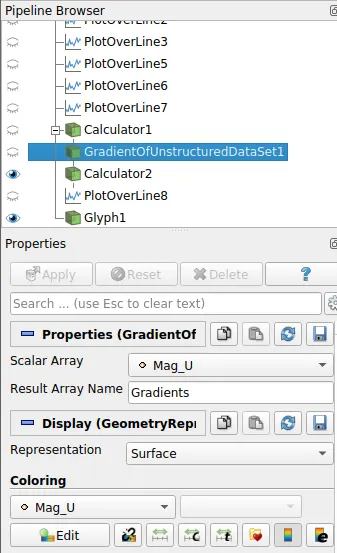
Using the calulator tool we make use of above relation calculate the Shear stress values.
Shear Stress across the C/S at location x = 0.0025 m from the Inlet -
Shear Stress across the C/S at location x = 2.32 m (Entry Length) from the Inlet -
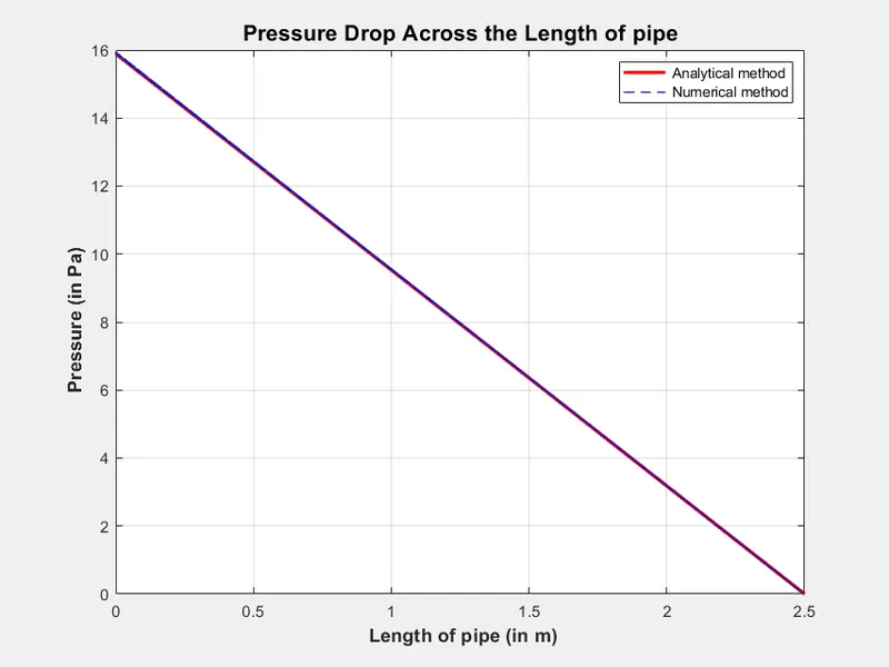
7. Validation of the Analysis by matching the Numerical results with Analytical Values -
Following is the MATLAB Code inorder to read the analysis data from .csv file and comparing with the analytical values -
clear all
close all
clc

% Input parameters

    % Reynold's Number
    Re = 2000;

    % Total Length of pipe(m)
    L = 2.5;

    % Diameter of pipe in meters
    D = 0.02;

    % Wedge Angle in degrees
    theta = input('n     Wedge Angle in degrees - ');

    % Density (kg/m^3)
    rho = 997;

    % Dynamic Viscosity (Pa.sec)
    mu = 8.90e-4;

    % Radius of pipe(m)
    R = D/2;

    % Entrance Length
    Le = 0.058*Re*D;

%--------------------------------------------------------------------------
% Calculations for Analytical methods
%--------------------------------------------------------------------------

% Average Velcity
Vavg = (Re*mu)/(rho*D);

% Velocity Profile at c/s from center to te wall of the pipe in fully developed region
    r = linspace(0,R,1000);
    Vr=2*Vavg*(1-(r.^2/R^2));
    % Velocity at center
    Vmax = 2*Vavg;


% Pressure Drop in across the length of pipe
    L_an = linspace(0,L,1000);
    P_drop = (32*mu.*L_an.*Vavg)/D^2;
    P_drop = fliplr(P_drop);


% Wall Shear Stress
    % Darcy Friction Factor
    f = 64/Re;
    % wall Shear stress
    tau_w = (f/4)*((rho*Vavg^2)/2);


%--------------------------------------------------------------------------
%   Retriving OpenFOAM Analysis Data from CSV Files
%--------------------------------------------------------------------------

    % Reading Velocity File Extracted from paraView
    fv = fopen('Velocity_Profile_of_Fully_Developed_Flow_at_Entry_Length.csv','r');
    fgetl(fv);
    for i = 1:1000
        C = fgetl(fv);
        D = strsplit(C,',');
        Vn(i) = D(1);
        Lr(i) = D(6);
    end
    Vn = str2double(Vn);
    Lr = str2double(Lr);


    % Reading Pressure File Extracted from paraView
    fp = fopen('Pressure_Drop_across_the_Pipe.csv','r');
    fgetl(fp);
    for i = 1:31685
        C = fgetl(fp);
        D = strsplit(C,',');
        Pn(i) = D(1);
        Lp(i) = D(5);
    end
    Pn = str2double(Pn);
    Lp = str2double(Lp);


%--------------------------------------------------------------------------
%   Plotting the comparison
%--------------------------------------------------------------------------

% Velocity comparison from analytical method and numerical method
figure(1)
    set(gcf, 'Position',  [100, 200, 800, 600])
    plot(r,Vr,'color','r','linewidth',2)
    hold on
    plot(Lr,Vn,'--','color',[0 0.1 0.8],'linewidth',2)
    xlabel(' Location or Radial Dist. from the center to wall of pipe (in m)','fontweight','bold','fontsize',12)
    ylabel(' Velocity (in m/s)','fontweight','bold','fontsize',12)
    title(' Velocity Profile comparison of analytical and numerical values','fontsize',14)
    legend(' Analytical method',' Numerical method')
    grid on

% Pressure comparison from analytical method and numerical method
figure(2)
    set(gcf, 'Position',  [905, 200, 800, 600])
    plot(L_an,P_drop,'color','r','linewidth',2.5)
    hold on
    plot(Lp,Pn,'--','color',[0 0.1 0.8],'linewidth',1)
    xlabel(' Length of pipe (in m)','fontweight','bold','fontsize',12)
    ylabel(' Pressure (in Pa)','fontweight','bold','fontsize',12)
    title('Pressure Drop Across the Length of pipe','fontsize',14)
    legend(' Analytical method',' Numerical method')
    grid on


% Error
    err_max = max(max(abs(Vr-Vn)));
fprintf('n t Max. Error of velocity Profile between Analytical & Numerical Result = %f n',err_max); 
RESULTS & CONCLUSION :
- Following are the Results from Analyitical calculation and Simulation,

- We can see above the the Error between analytical values and Numerical simuation values is very small. And satisfies with the pressure drop value calculated with Hagen-Poiseuille Equation.
- Hence, the Simulation of Laminar/Hagen-Poiseuille Flow through pipe is successful and satisfactory.
- Smart Techiniques like here using axis-symmetric nature of the flow, and doing simulation only for a small sector Cross-section of the pipe; shows how can a CFD problem project can be optimized to have comparitively less computation power and time while getting the required & reliable results.
REFERENCE :
- https://atomstalk.com/blogs/the-poiseuille-equation/#The_Equation
- https://en.wikipedia.org/wiki/Entrance_length_(fluid_dynamics)
- https://www.youtube.com/watch?v=3eugpW5pBnY&ab_channel=Spoken-TutorialIITBombay
- https://openfoamwiki.net/index.php/Main_ContribExamples/AxiSymmetric
- https://www.tec-science.com/mechanics/gases-and-liquids/hagen-poiseuille-equation-for-pipe-flows-with-friction/
- https://www.simscale.com/docs/validation-cases/hagen-poiseuille-flow/