Week 5.1 - Non-Conformal Meshing and Solving a Cold plate model

AIM : To create a Non-Conformal mesh for the Cold Plate Model and Solving the Case in Ansys Icepak model.

OBJECTIVES :

• Create the Cold Plate Model Geometry and setup in Icepak
• Making the Non-Conformal meshing for the given Case.
• Setup the model for the Analysis.
• Run the simulation and Post Process the results.

INTRODUCTION :

A non-conformal mesh, when there are a partial or zero matchings of nodes at the interface. This means that one, few, or every node on one side of the interface doesn't have a match on the other side of the interface.

STEPS / PROCEDURE :

1) Creating Geometry and Assigning their Properties & Boundary Conditions

Following are the Geometry creation and assignments as given in the Case -

a. Cabinet

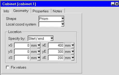
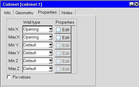
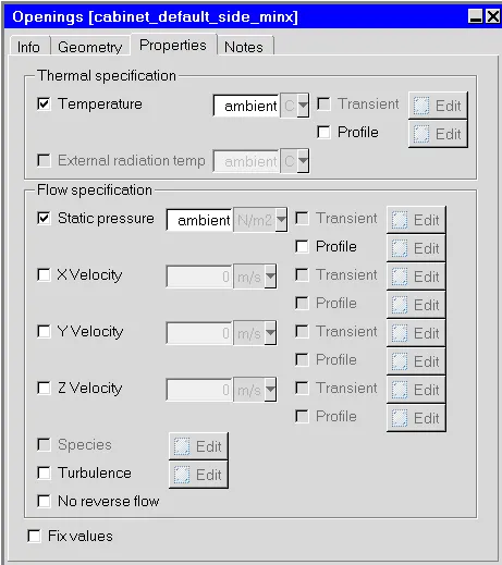
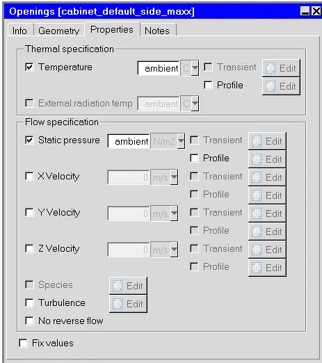
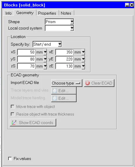
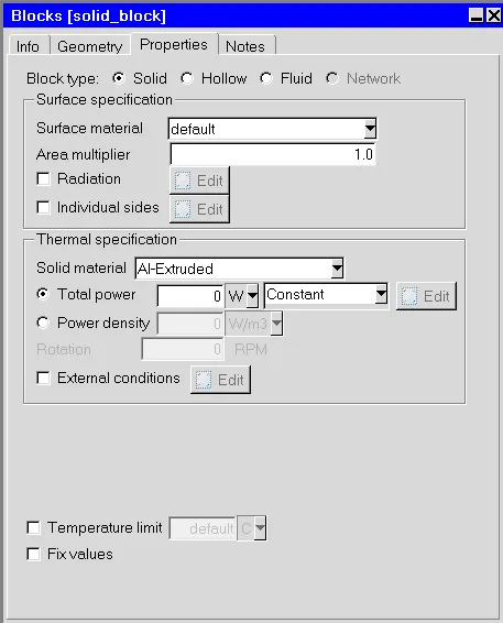
b. Solid Block

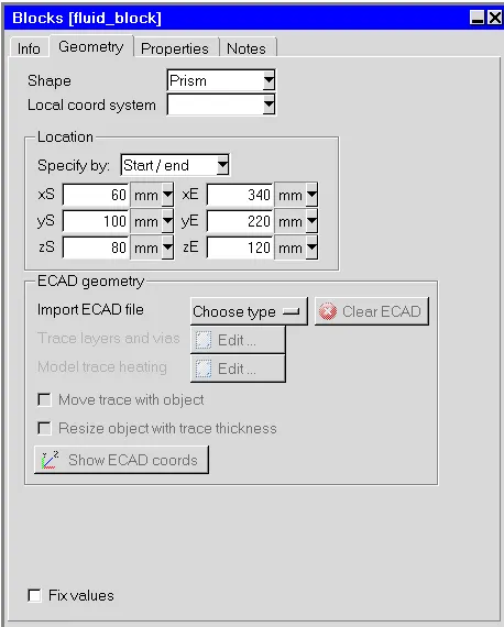
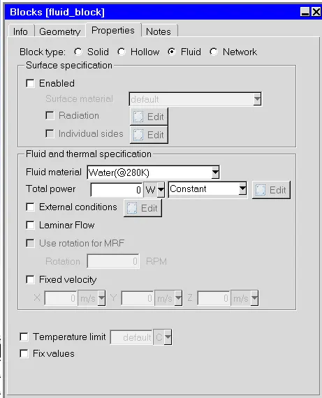
c. Fluid Block

d. Fluid Inlet

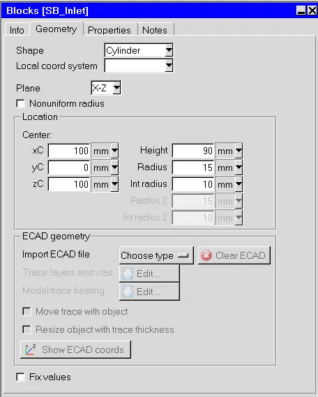
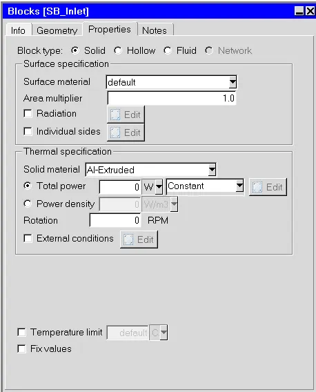
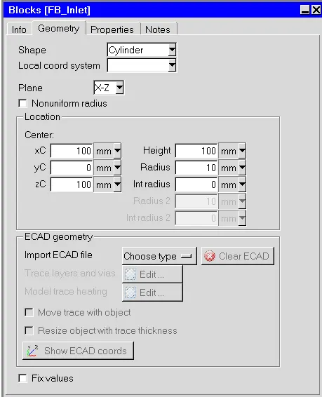
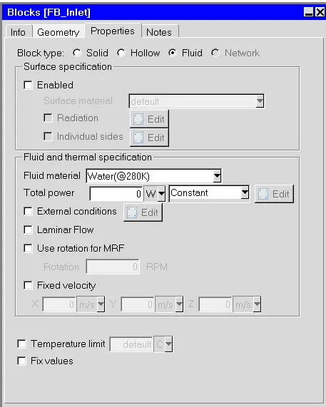
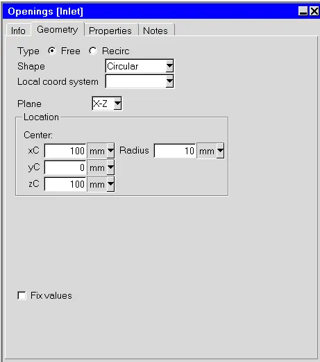
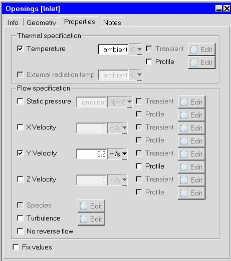
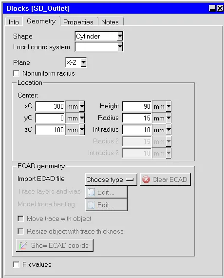
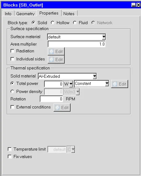
Setting up for For fluid inlet and outlet there is 3 things create; solid body of pipe, Fluid Volume of pipe & the opening for the entry and exit.

Solid Body for the Inlet -

Fluid Volume for Inlet -

Opening for Inlet -

e. Fluid Outlet

Solid Body for the Outlet -

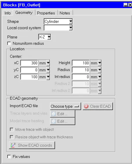
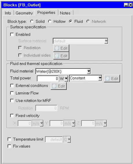
Fluid Volume for Outlet -

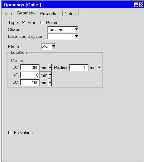
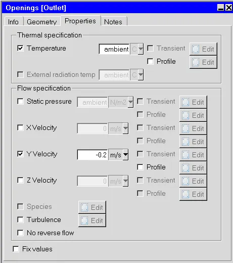
Opening for Outlet -

f. Heat Plates

Heat Plates are the sources of heat in this case of simulation.

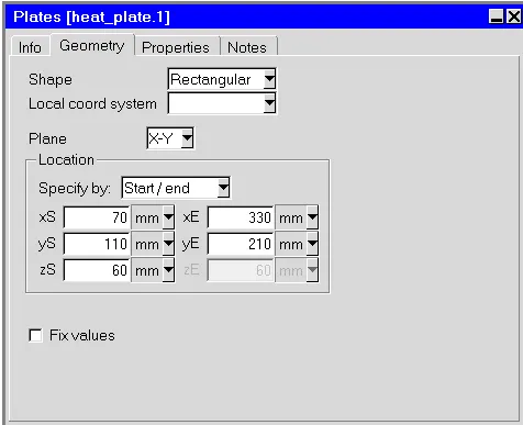
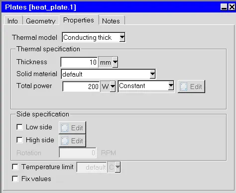
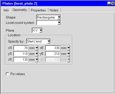
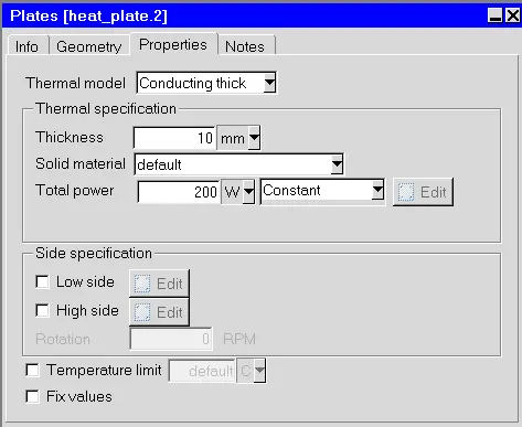
The Following is the Case Geometry Generated -

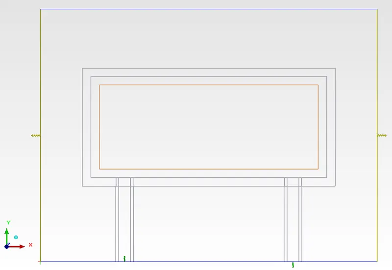
2) MESHING

Following is the Global Mesh Setting we are using, which we discussed earlier in Conformal Meshing.

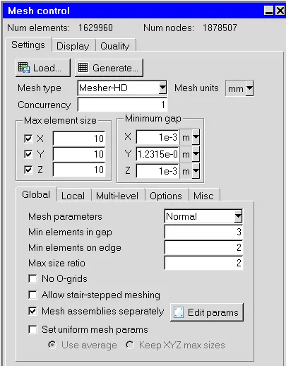
Now, For this Project our main goal to simulate the case using Non-Conformal meshing. For non-conformal meshing, it is important have different assemblies, and we make non-conformal mesh by meshing the each Assembly separately.

Following are the Different Mesh assembly created and their Mesh Settings -

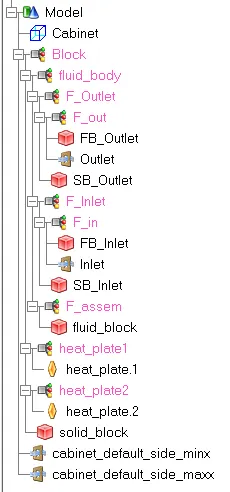
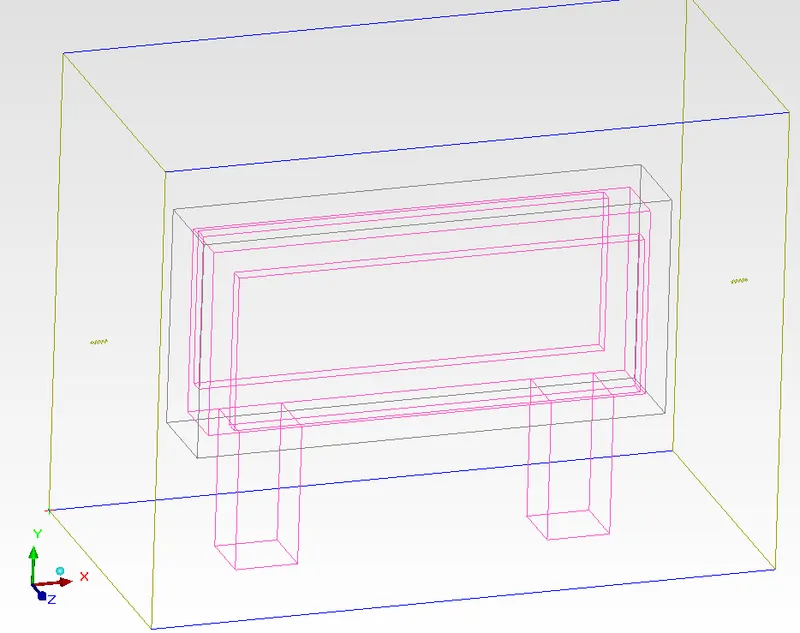
Following are the Assembly mesh settings listed in above picture -

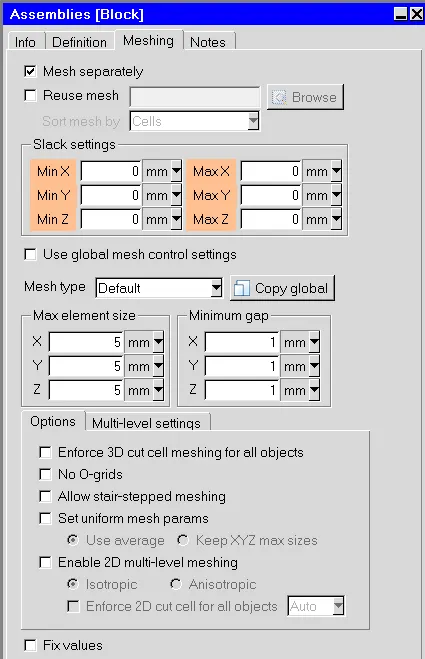
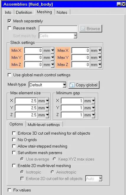
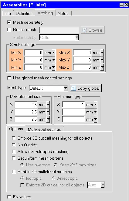
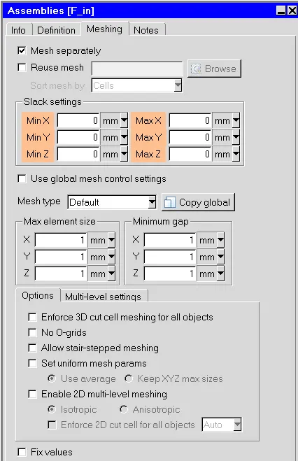
(Same Settings for Outlet pipe Assembly as above)

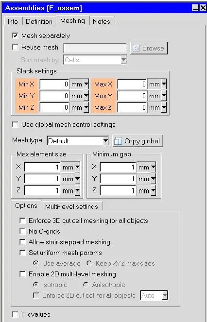
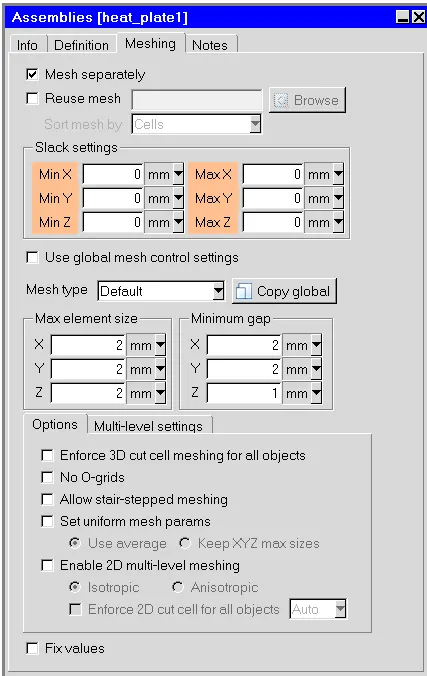
3) SOLVER SETUP

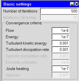
Basic parameters panel:

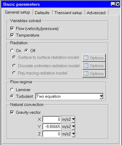
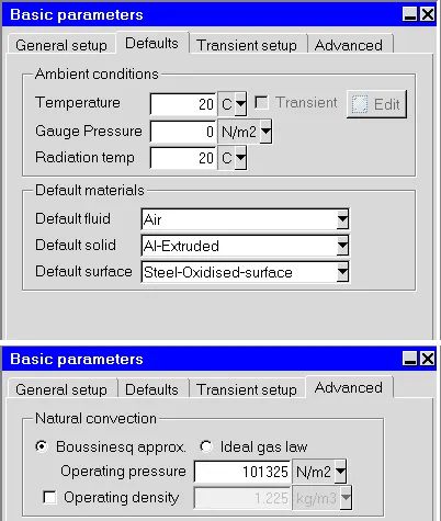
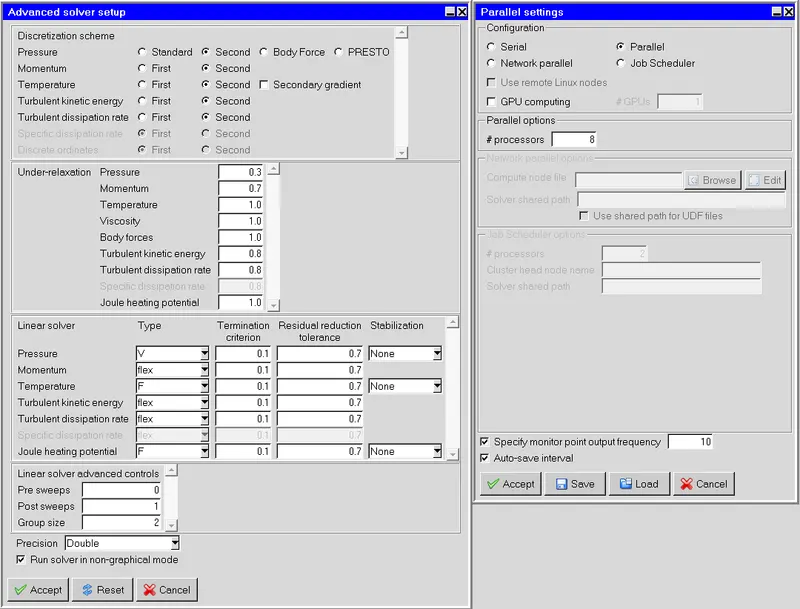
Basic and advanced settings panel:

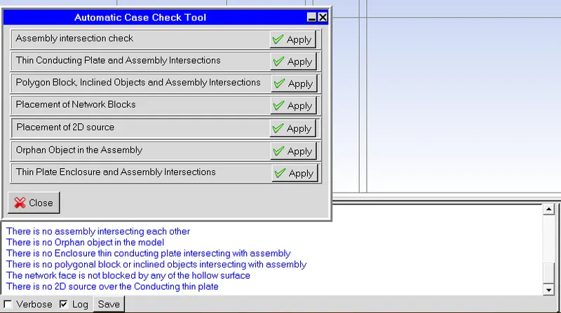
Macros Mesh Checking -

POST-PROCESSING :

i) Generated mesh.

Following is the surface mesh of the Cold Plate Case Setup.

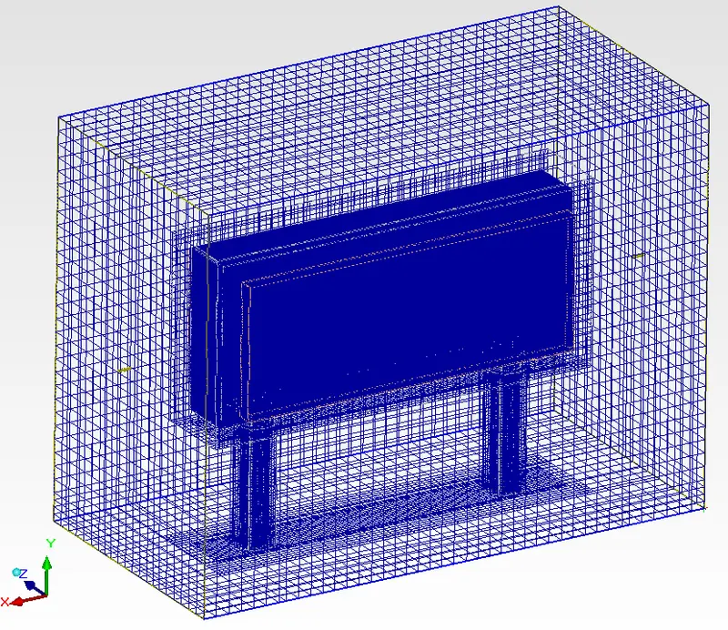
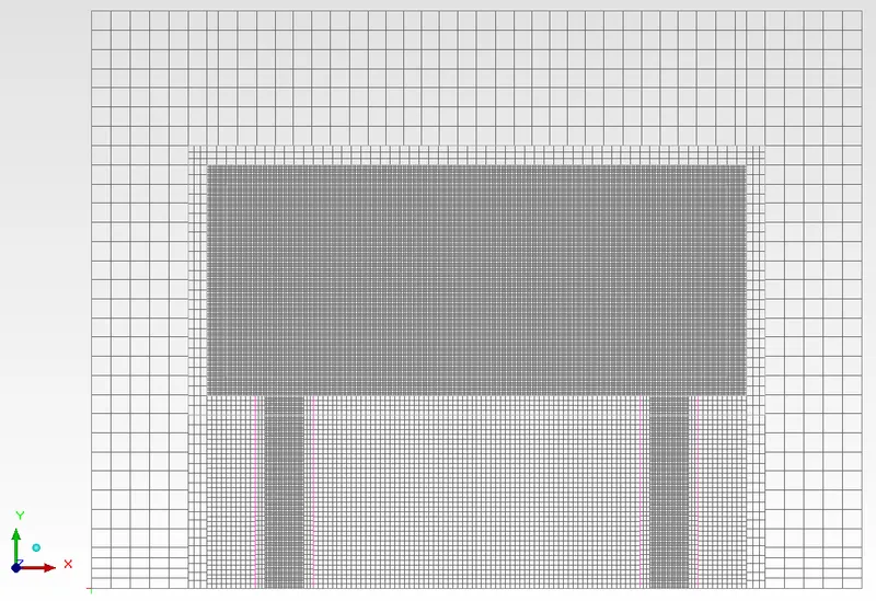
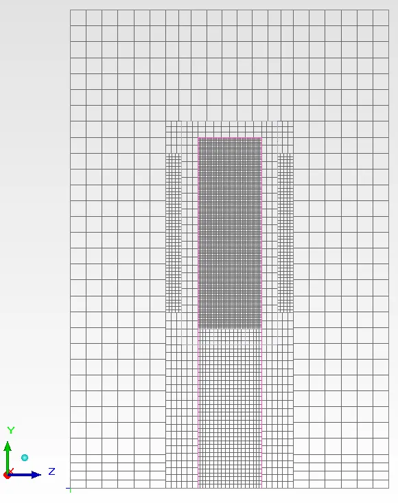
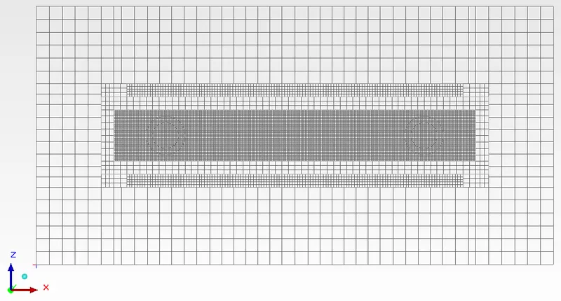
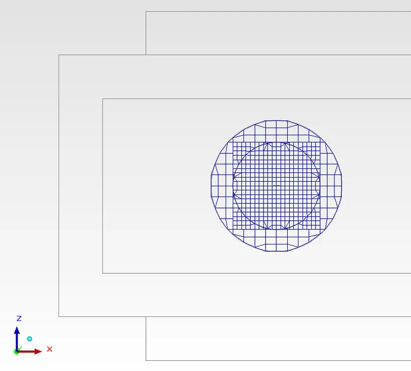
Following is the visualising the mesh inside the cabinet-

- Cut plane of XY plane at 50% of the cabinet in Z-direction from origin (Top Plane)

- Cut plane of YZ plane at 50% of the cabinet in X-direction from origin (Front Plane)

- Cut plane of XZ plane at 50% of the cabinet in Y-direction from origin (Right Plane)

- C/S View of Mesh at the Pipes's Solid Block, Fluid Block and Opening.

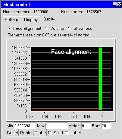
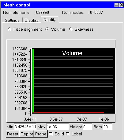
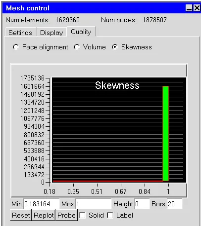
Mesh Quality

Following are the mesh quality for the respective parameters i.e., Face Alignment, Volume and Skewness.

ii) Outputs

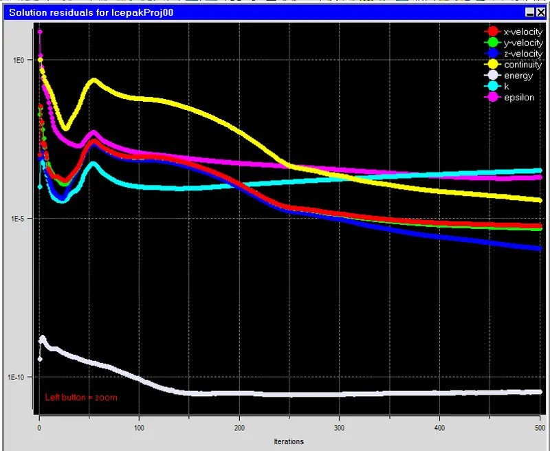
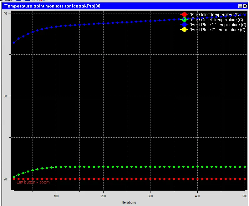
Residuals and Monitor Points -

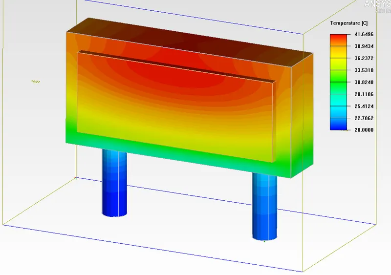
Temperature Contours -

Face plot over the Solid Bodies -

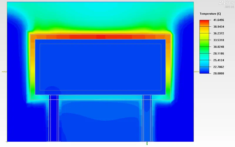
Cut plane of YZ plane at 50% of the cabinet in X-direction from origin (Front Plane)

- Cut plane of XZ plane at 50% of the cabinet in Y-direction from origin (Right Plane)

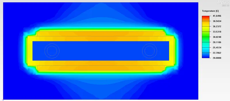
- Cut plane of XZ plane at 50% of the cabinet in Y-direction from origin (Right Plane)

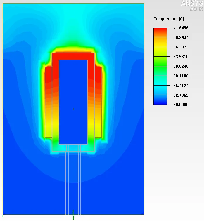
From the temperature contours from different views we can see the hot spot of the temperature and temperature distribution inside the cabinet and bodies. We can also see the temperature of liquid coolant and also of the air natural convection.

Velocity Contours

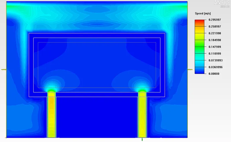
Streamline Visulization of Velocity for the liquid cooling -

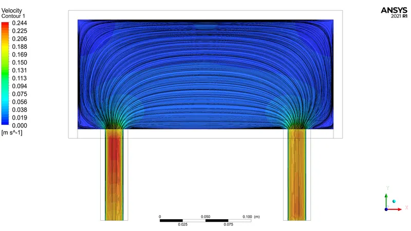
From above figures we can see the contour showing the velocity of the fluid at different locations inside the cabinet. And from the streamline(or Particle trace inside ICEPAK) we can see the flow path i.e. streamlines of the liquid coolant flowing inside.

RESULTS :

The Following are the results of the simulation, generated simulation report from the ICEPAK software Showing Various characteristic values of the simulation and the max. temperatures of the different bodies acting in the simulation -

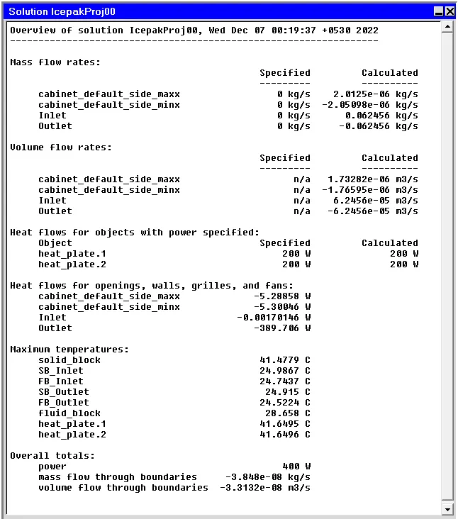
The maximum temperature within the computational domain is 41.6496 deg.C. at the heatplates.
The maximum air velocity within the computational domain is 0.295997 m/s.

CONCLUSION :

Hence, We have completed the simulation for the cold-plate case using Non-Conformal meshing.

We can see the temperatures attained are realistic and all the residuals are less than 10e-3.

Also, we have seen different Contour & streamline visualization of temperatures and velocity .