Program to Solve an OTTO Cycle, Plot P-V Diagram and calculates Engine Thermal Efficiency using MATLAB. (Matlab/Challenge-Week 2-Air standard Cycle)
Theory :
An Otto cycle is an idealized thermodynamic cycle that describes the functioning of a typical spark ignition piston engine. It is the thermodynamic cycle most commonly found in automobile engines. It tells what happens to a mass of gas as it is subjected to changes of pressure, temperature, volume, addition of heat, and removal of heat. The mass of gas that is subjected to those changes is called the system. The system, in this case, is defined to be the fluid (gas) within the cylinder.
It can be visualised from the following diagram -
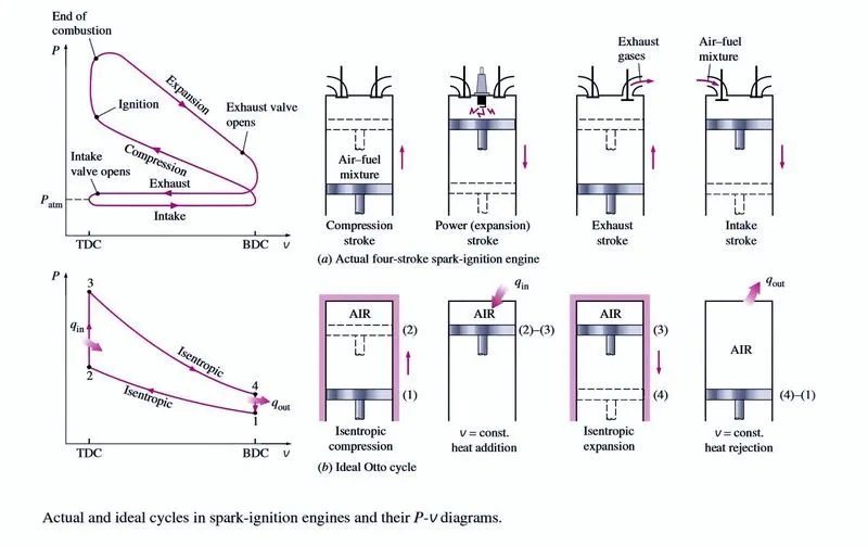
OTTO Cycle Consists of Four main processes -
i) Isentropic Compression (1-2)
ii) Constant Volume Heat Addition (2-3)
iii) Isentropic Expansion (3-4)
iv) Constant Volume Heat Rejection (4-1)
These processes are governed by the following thermodynamic equations -
a) For Isentropic Processes:
`p_2.v_2^gamma = p_1.v_1^gamma`
`(p_2.v_2)/t_2 = (p_1.v_1)/t_1`
[Note: Considering 1 to 2 be any consecutive isentropic process]
b) For Constant Volume Processes:
`v_2 = v_1`
`(p_2)/t_2 = p_1/t_1`
[Note: Considering 1 to 2 be any consecutive isochoric process]
Now from these above governing equations we can find the state variables at the states 1,2,3 & 4.
Thermal Efficiency: In general the thermal efficiency, `η_(th)`, of any heat engine is defined as the ratio of the work it does, W, to the heat input at the high temperature, `Q_i`.
`eta_(th) = W/Q_i = (Q_i-Q_o)/Q_i =1 - Q_o/Q_i`
`=> eta_(th) = 1 - (T_4-T_2)/(T_3 -T_2)`
Where, W = Work done or work output
`Q_i` = Heat Added to the system (Input)
`Q_o` = Heat Rejected or Wasted (Output)
`eta_(th)` = Thermal Efficiency
A state variable in a thermodynamic system is defined by any two variables out of Temperature(T), Pressure(P), volume(V) and Entropy(S). and presented in either P-V diagram or T-S Diagram.
In this, we are focusing on the P-V Diagram for solving and representing OTTO Cycle. Therefore, our main concern is on finding the Pressure, Volume and Temperature of the state.
Now for this graph by the given parameters and volume of a cylinder, we can calculate only the Endpoint states of the processes i.e. 1,2,3 & 4, which will give straight lines between the endpoints. but a process has several state points corresponding to piston positions between the end-state points and each have different in state variables properties.
Therefore, here Engine(or piston) kinematics comes into play. To solve this problem we trace the volume of the cylinder at each piston position between TDC and BDC.
This is done by the following equation -
`v/v_c = 1 +1/2*(r_c-1)*[ R + 1 - costheta - (R^2 - sin^2theta)^0.5]`
where, v = volume corresponding to the piston position
`r_c` = Compression ratio
a = crank pin radius
R = ration of connecting rod to crank pin radius
`V_c =` Clearance volume
`V_s =` Swept volume
Some important terms -
-> `a = (Stroke)/2`
-> R = (Connecting Rod length) `/a`
-> `v_s = pi/4*(BORE)^2*STROKE`
-> `v_c = v_s/(r_c-1)`
Program :
- Following is the program's Main function which computes and plots the OTTO Cycle -
%_______________________________ Program for OTTO Cycle ___________________________ clear all close all clc % GIVEN t1 = 500; % temperature are in Kelvin p1 = 101325; % pressure in Pa t3 = 2300; gamma = 1.4; % Engine geometric parameters bore = 0.1; stroke = 0.1; con_rod = 0.15; cr = 12; % calculating volumes v_swept = (pi/4)*bore^2*stroke; v_clearance = v_swept/(cr-1); v1 = v_swept + v_clearance; v2 = v_clearance; %------------------- Variables at State 2 for Process 1-2 (COMPRESSION) ------------------- % p2.(v2^gamma) = p1.(v1^gamma) % p2 = p1.(v1/v2)^gamma p2 = p1*(cr^gamma); % (p2.v2)/t2 = (p1.v1)/t1 t2 = (p2*v2*t1)/(p1*v1); v_compression = engine_kinematics(bore, stroke, con_rod, cr, 180, 0); p_compression = (p1*(v1^gamma))./(v_compression.^gamma); %------------------- Variables at State 3 Process 2-3 (CONSTANT VOLUME HEAT ADDITION)------------------- v3 = v2; % (p3.v3)/t3 = (p2.v2)/t2 % since v3 = v2, % Therefore, p3 = p2.(t3/t2) & t3 = 2300 p3 = (p2*t3)/t2; %------------------- Variables at State 4 Process 3-4 (EXPANSION) ------------------- v4 = v1; % p3.(v3^gamma) = p4.(v4^gamma) % p4 = p3.(v3/v4)^gamma p4 = p3*(v3/v4)^gamma; % (p4.v4)/t4 = (p3.v3)/t3 t4 = (p4*v4*t3)/(p3*v3); v_expansion = engine_kinematics(bore, stroke, con_rod, cr, 0, 180); p_expansion = (p3*(v3^gamma))./(v_expansion.^gamma); figure(1) hold on; grid on; title('P-V Diagram of OTTO Cycle'); xlabel('Volume'); ylabel('Pressure'); plot(v1,p1,'-k.','MarkerSize',15); plot(v_compression,p_compression,'color','r','linewidth',2); % Isentropic Compression Process plot(v2,p2,'-k.','MarkerSize',15); plot([v2 v3],[p2 p3],'color','m','linewidth',2); % Constant Volume Heat Addition Process plot(v3,p3,'-k.','MarkerSize',15); plot(v_expansion,p_expansion,'color','b','linewidth',2); % Isentropic Expansion Process plot(v4,p4,'-k.','MarkerSize',15); plot([v4 v1],[p4 p1],'color','g','linewidth',2); % Constant Volume Heat Rejection Process legend('Temp. T1','Isentropic Compression','Temp. T2','Constant Volume Heat Addition Process',... 'Temp. T3','Isentropic Expansion Process','Temp. T4','Constant Volume Heat Rejection Process') te = 1-((t4-t1)/(t3-t2)); % Thermal Efficiency tep = te*100; fprintf('Thermal Efficiency of the Engine : %f',te) fprintf(' = %f %% n',tep) - Following is function which traces the volume of the cylinder at different piston positions -
function [V] = engine_kinematics(bore, stroke, con_rod, cr, start_crank, end_crank) a = stroke/2; % Crank pin Radius R = con_rod/a; % Ratio of Connecting Rod length to Crank pin Radius v_s = (pi/4)*bore^2*stroke; % swept volume v_c = v_s/(cr-1); % clearance volume theta = linspace(start_crank, end_crank,180); % for volume trace equation - term1 = 0.5*(cr-1); term2 = R + 1 - cosd(theta); term3 = (R^2 - (sind(theta)).^2).^0.5; V = (1 + term1*(term2 - term3)).*v_c; end
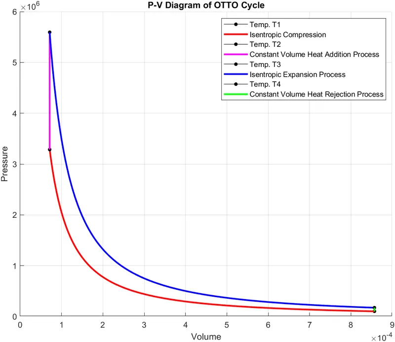
Output :
i) OTTO Cycle -
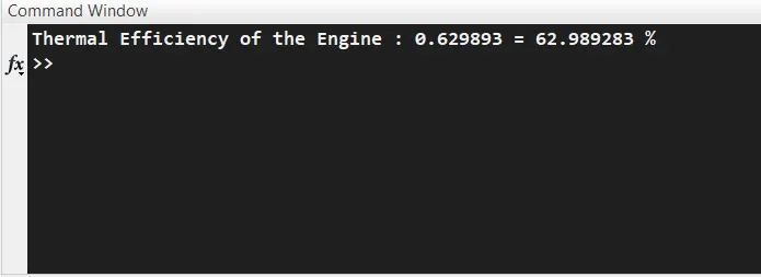
ii) Thermal Efficiency of the Engine -