Week 2 - Flow over a Cylinder.
AIM : To perform Simulation of Flow over a Circular Cylinder Different Reynold No. Flow for analyzing the Von Kármán vortex street Flow Behaviour and Strouhal number.
OBJECTIVES :
- Setting up the Geometry in Spaceclaim.
- Create optimal meshing for the model in Ansys Mesher.
- Setup the model for the analysis from the given data.
- Run the simulation and Post Process the results.
- Get Results For Reynolds No.s 10, 100, 1000, 10000, 100000 in steady state simulation.
- Simulate both steady state and transient simulation for the Re =100.
INTRODUCTION :
One of the classical problems in fluid mechanics is the determination of the flow field around a bluff body represented by a circular or rectangular cylinder. This is of great interest in many engineering applications, such as heat exchanger, chimney, hydrodynamic loading on ocean marine piles and offshore platform risers and support legs.
From scientific perspective, flow around a circular cylinder is having some important phenomenon of fluid dynamics, such as transition to turbulent, separation, and vortex shedding. From the following diagram we can see the flow characteristics over a circular cylinder surface. Boundary layer Formation, point of separation, and Wake Formation.
Laminar Boundary Layer ( Ref. [10] )
The different range of Reynolds Numbers represents different flow patterns. At low Reynolds Numbers, the flow pattern is observed to be Laminar i.e., Smooth, Constant fluid motion. At higher Reynolds Numbers the flow pattern is observed to be Turbulent i.e., Chaotic eddies, Vortices, and Flow instabilities. As shown in following example of nature,
Turbulent Von Karman Vortex flow of Cloud ( Ref. [11] )
Due to the large low-pressure at wake region there is formation of the Vortices from backflow of the fluid. These vortices moves forward in the downstream and then these vortices get bigger due to diffusion. And this cause wake to grow and creat instabilities which can travel upstream and leads to vortex shedding.
( Ref. [1] )
There are two approximately parallel shear layers behind a bluff body such as a cylinder. On the outside, the flow goes forwards. On the inside, it goes backwards. This situation is even more unstable than a single shear layer. The shear layers start by snaking up and down together. Soon they roll up into vortices that are shed alternately from each side of the cylinder. This is vortex shedding.
The vortex shedding frequency, f , is a function of the speed of the flow, V, and the distance between the shear layers, D. Experimentally one finds that the Strouhal number, f.D/V , is approximately 0.2 at moderate and high Reynolds numbers. Vortex shedding has important consequences for structures such as chimneys, particularly if the frequency of vortex shedding matches the resonant frequency of the structure.
( Ref. [1] )
In fluid dynamics, a Kármán vortex street (or a von Kármán vortex street) is a repeating pattern of swirling vortices, caused by the vortex shedding.
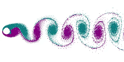
(Source: Wikipedia)
A vortex street will form only at a certain range of flow velocities, specified by a range of Reynolds numbers (Re). The (global) Reynolds number for a flow is a measure of the ratio of inertial to viscous forces in the flow of a fluid around a body or in a channel, and may be defined as a nondimensional parameter of the global speed of the whole fluid flow :
`R_e = (U*L)/nu` or `R_e = (rho*U*L)/mu`
where, `R_e =` Reynold's Number
`L =` Characteristic Length parameter of the body or channel
`U =` Free Stream Flow speed of the Fluid
`rho =` Density of the Fluid
`mu =` Kinematic Viscosity of the Fluid
`nu =` Dynamic Viscosity of the Fluid
From the Following Diagram, We can see the different Flow behaviour and Vortex Street at different Reynold's No. range across a circular cylinder :
Flow Regime of Fluid Flow Across a Smooth Tube
The Strouhal number is a dimensionless number describing oscillating flow mechanisms. It represents the ratio of inertial forces due to the local acceleration of the flow to the inertial forces due to the convective acceleration.
St = f . D / V
where
f = frequency of vortex shedding.
L = characteristic length (for example, hydraulic diameter or the airfoil thickness).
U = flow velocity.
STEPS / PROCEDURE :
1) Geometry
The Following is the geometry based on given dimensions in spaceclaim -
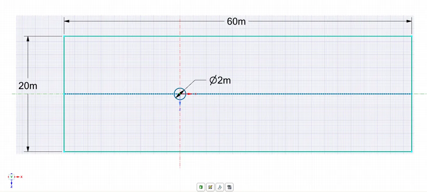
Here,
The Diameter of the cylinder, D = 2 m
For the good results the,
Length of the Domain = 30 x D
Breadth of the Domain = 10 x D
2) Meshing
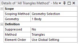
After doing Geometry preparation, we gone open the geometry in Ansys Mesher via workbench -
- Creating Named Selections
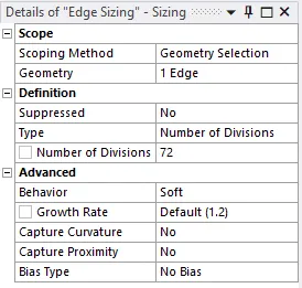
- Assigning proper mesh sizing
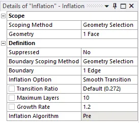
- Creating Inflation layers at the surrounding of the cylinder wall
- Checkng mesh quality.
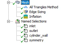
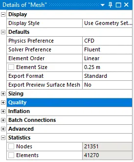
Mesh Quality Verification-
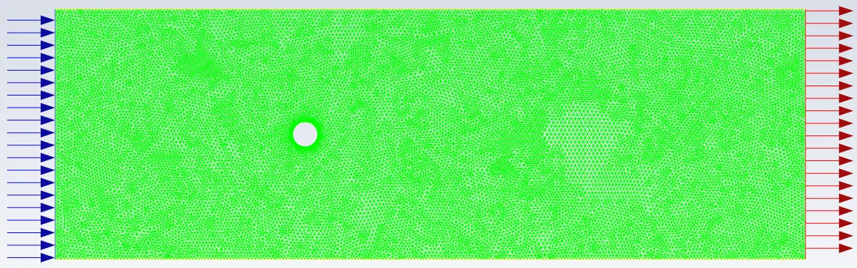
Following is the surface mesh of the Case Setup -
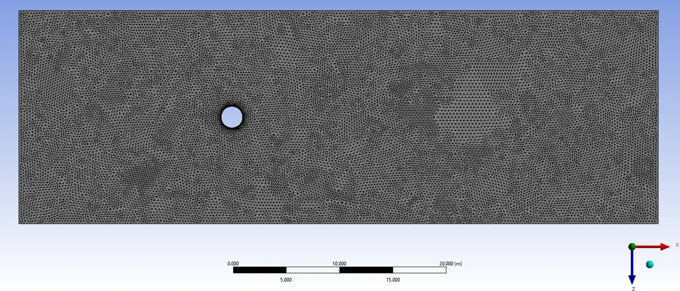
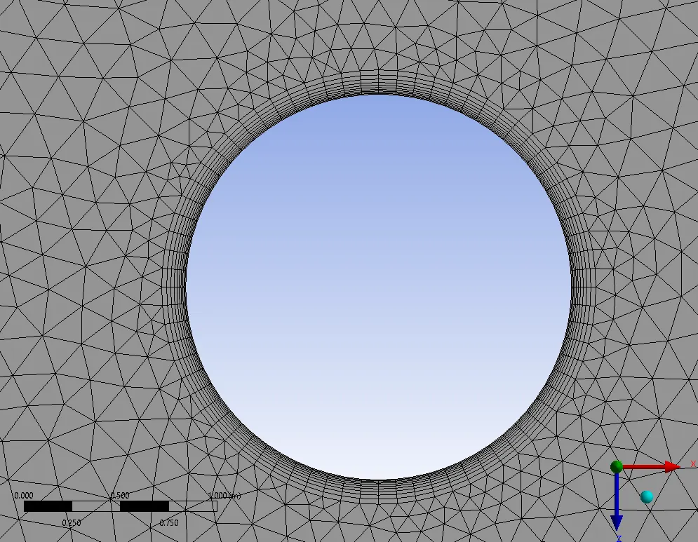
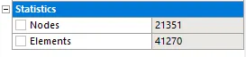
Mesh Quality -
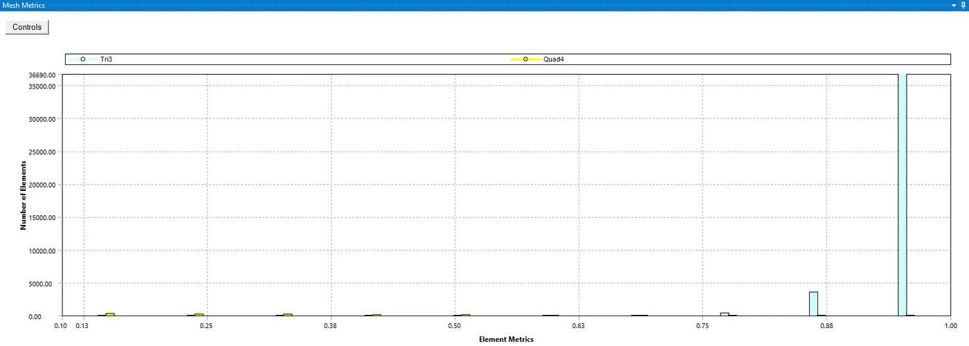
We can the mesh quality is very satisfied. 90% of the mesh cell are lying on good quality range.
3) Solver Settings -
Closing the Mesher & opening the Fluent Solver from the workbench
Checking the the Double precision option and selecting no. of parallel process.
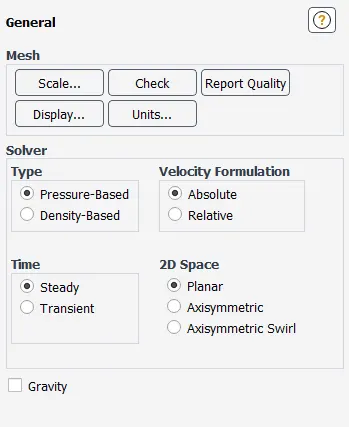
Setting solver settings and initialization values.
Currently we solving it in pressure based solver because there's negligible change in density.
Selecting the turbulence model and its settings.
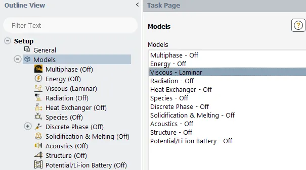
Now assigning the boundary conditions inlets, outlet, and walls.
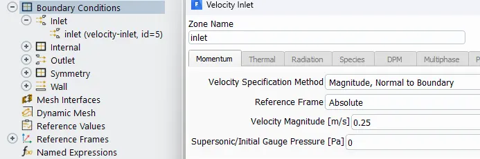
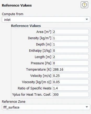
Reference Values for the Solution should computed from the inlet after assigning all properties and Boundary conditions.
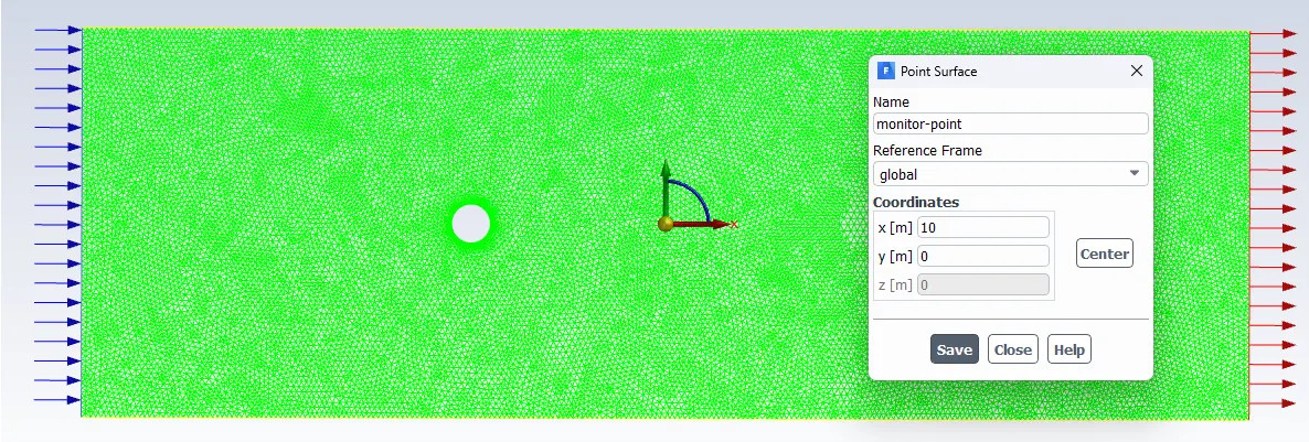
Creating Monitor point
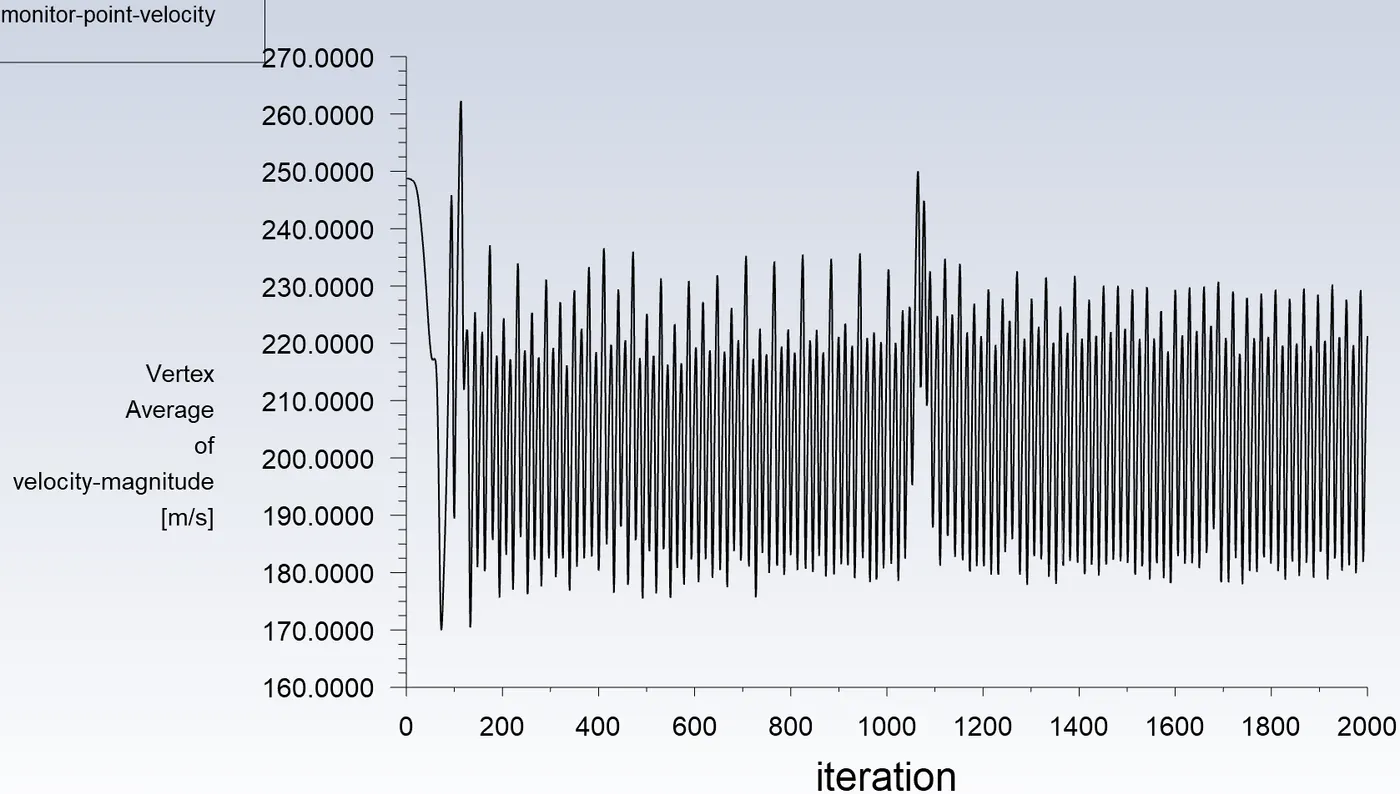
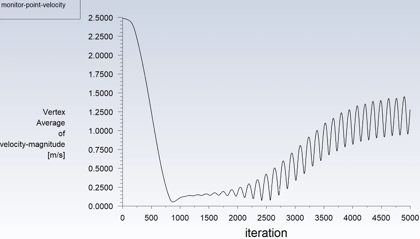
A monitor point is created at the distance 4 times the Diameter along the downstream to monitor the velocites and the passing vortices, which will be useful to calculate the frequency of the vortex street.
Setting Inilization, here we are using Hybrid Initialization.
Creating Solution reports.
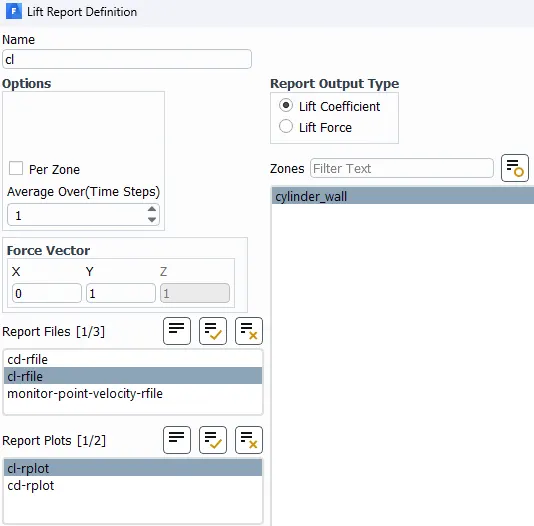
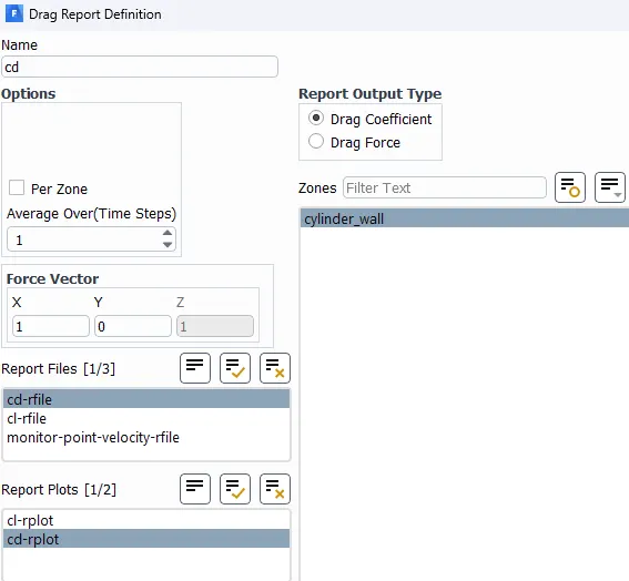
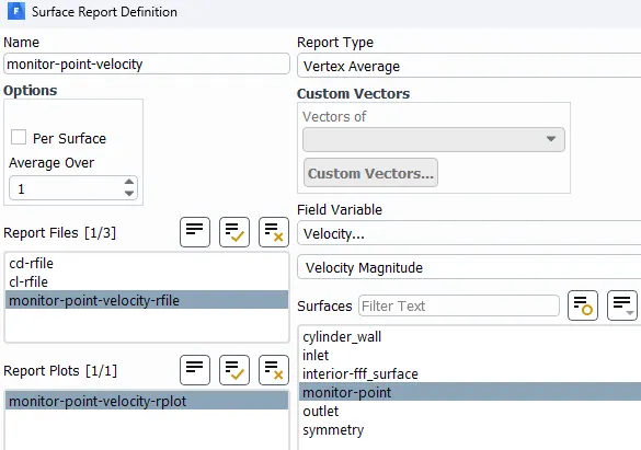
The convergence criteria has been turned off since we have monitor flow with respect to time.
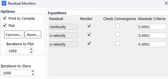
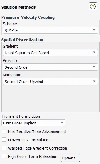
Keeping the Solution method & discretization schemes as shown below.
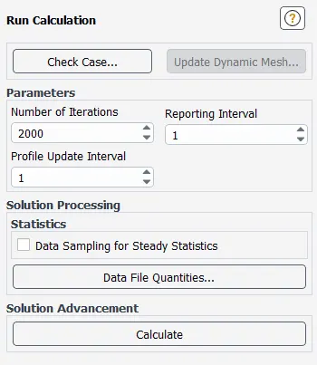
After Running the calculation we can plot strouhal no.
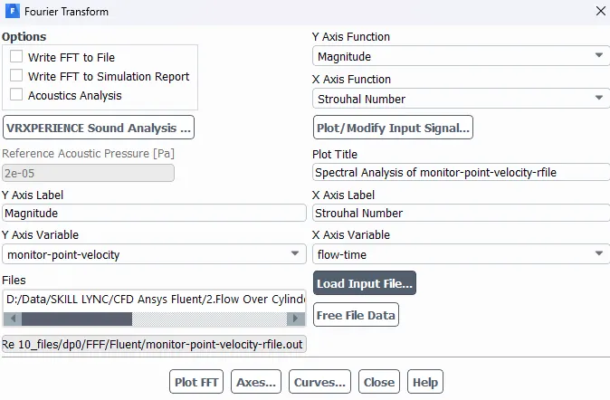
One write FFT to File and use avergare inorder to calculate the Strouhal no. using Ansys fluent.
For all other reynolds no. only the velocities will change and rest of the settings will remain same.
| Reynolds No. | Velocity ( in m/s ) |
| 10 | 0.25 |
| 100 | 2.5 |
| 1000 | 25 |
| 10000 | 250 |
| 100000 | 2500 |
For the Transient simulation for the Re = 100,
Following things will change and rest of the settings will remain same.
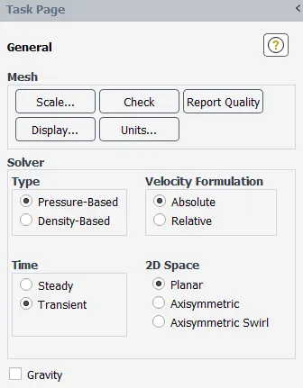
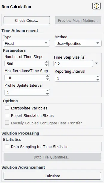
In the Calculation panel, for the transient simulation, total no. of timesteps are kept to 500 and timestep size is kept 0.2 Sec, therefore the We are simulating the flow over the cylinder upto 100 seconds.
And the 10 Iterations are kept for solving each time step.
POST PROCESSING :
Outputs
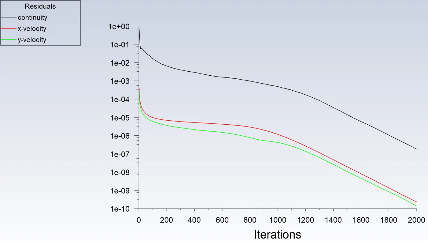
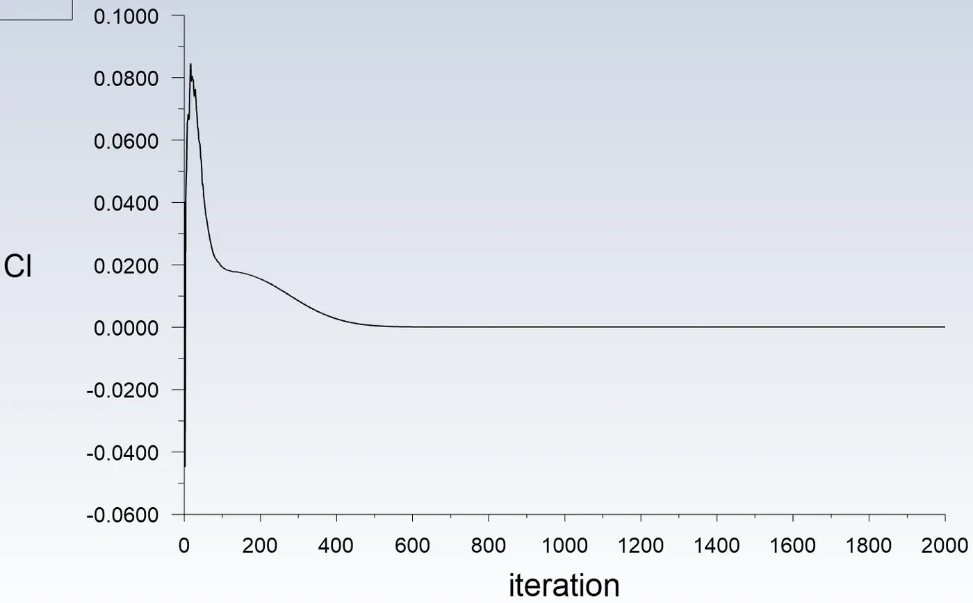
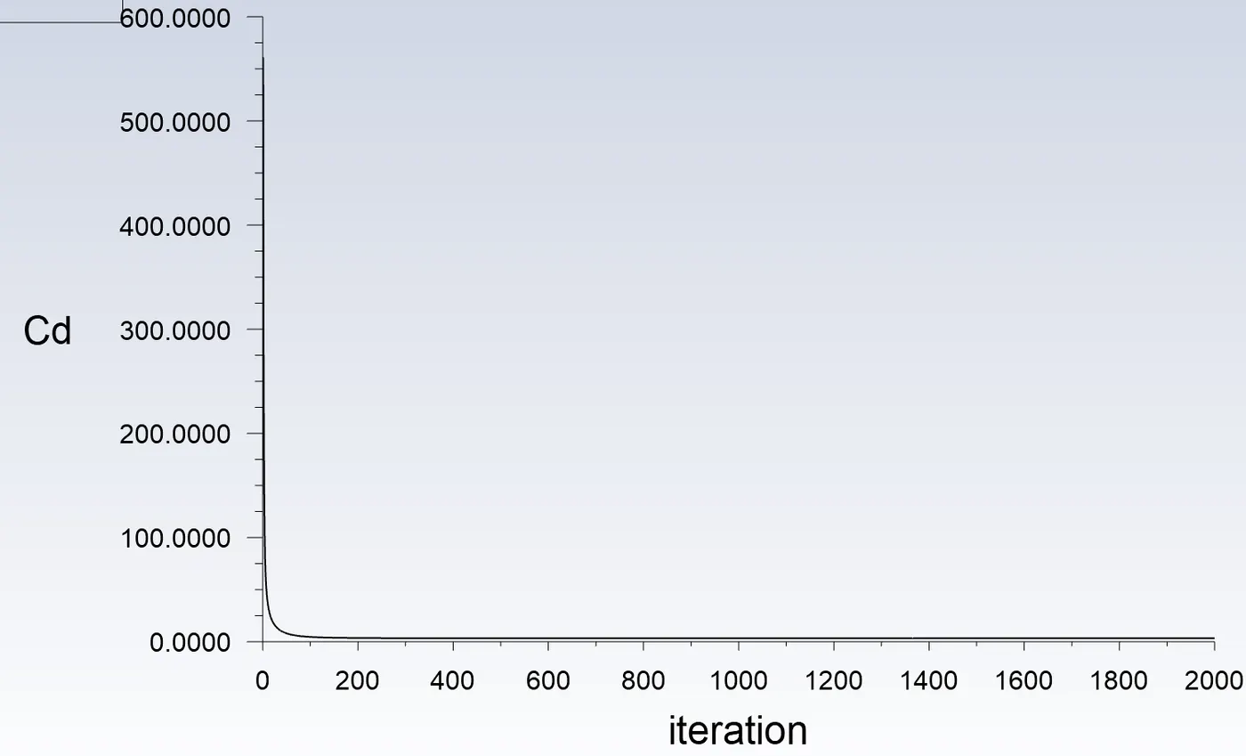
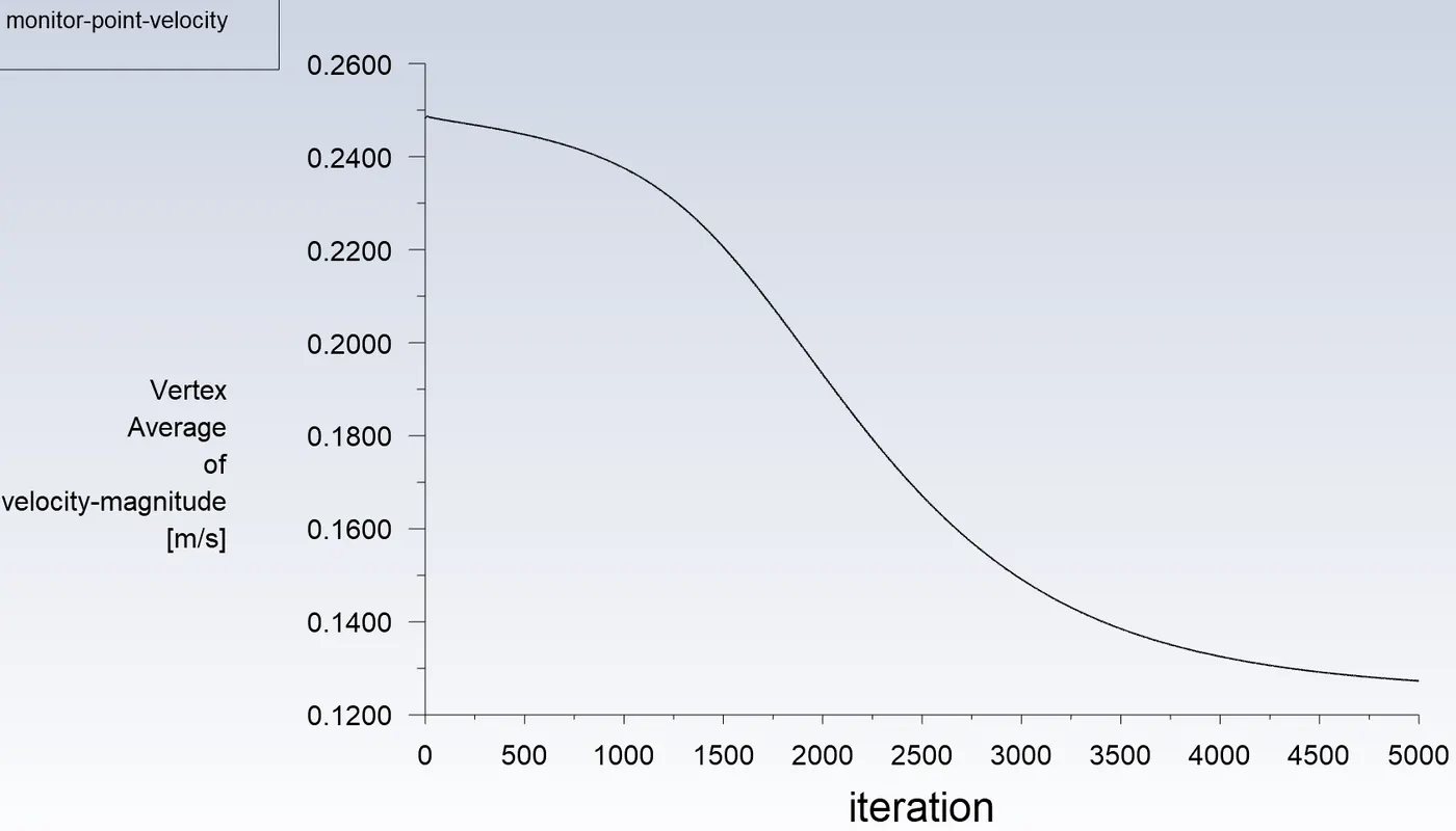
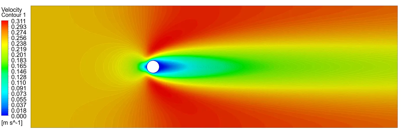
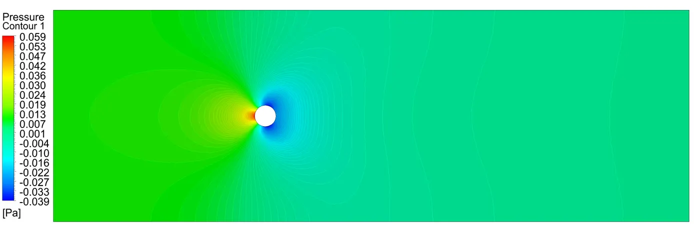
1. Steady State Analysis For Re = 10 -
Residuals and Solution Monitor Plot -
Contour Plots -
Velocity Contour -
Pressure Contour -
2. Steady State Analysis For Re = 100 -
Residuals and Solution Monitor Plot -
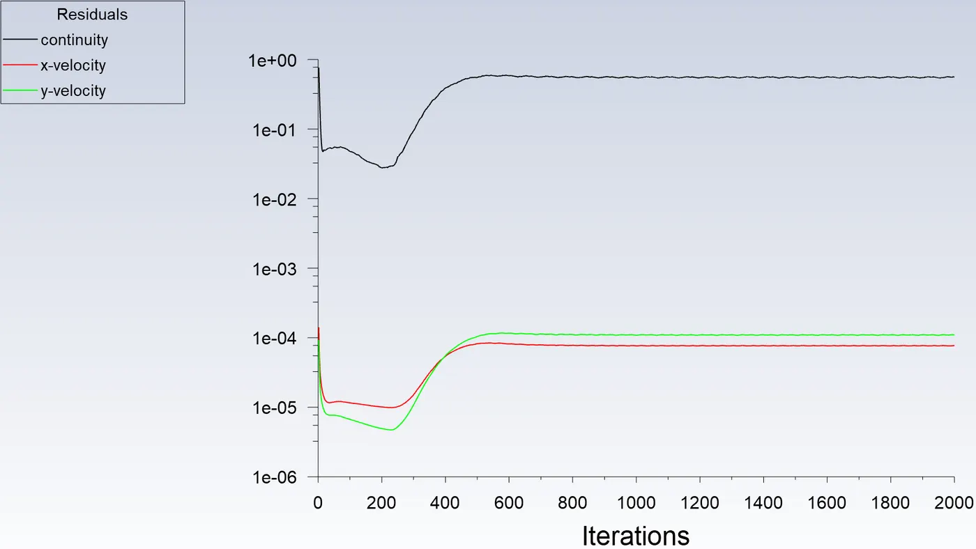
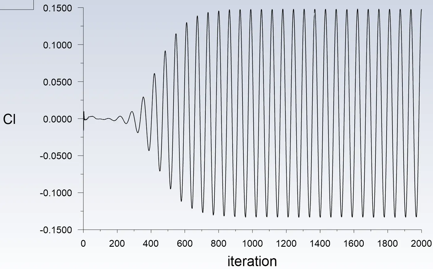
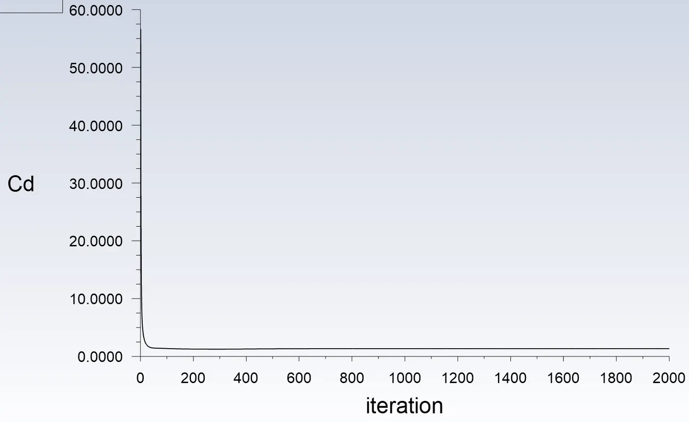
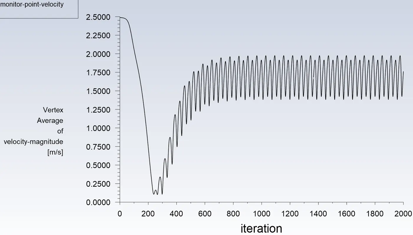
Contour Plots -
Velocity Contour -
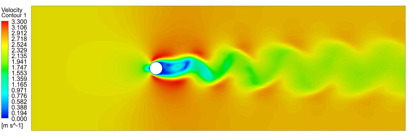
Pressure Contour -
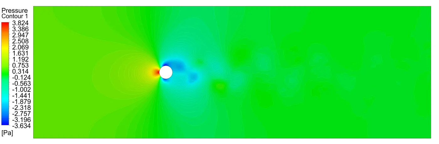
3. Steady State Analysis For Re = 1000 -
Residuals and Solution Monitor Plot -
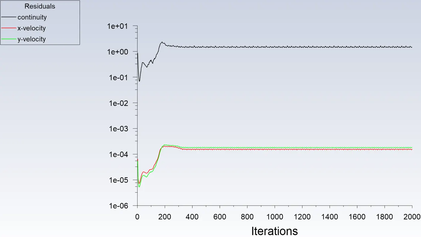
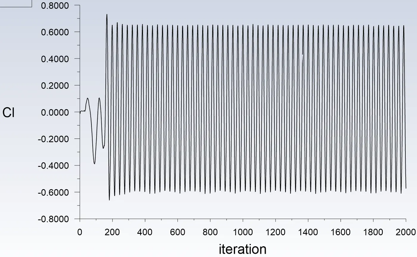
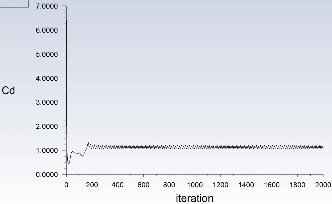
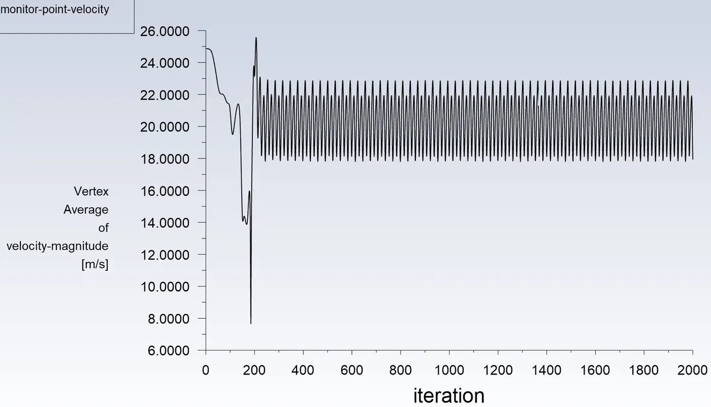
Contour Plots -
Velocity Contour -
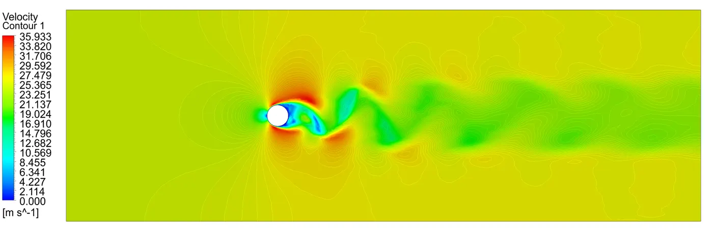
Pressure Contour -
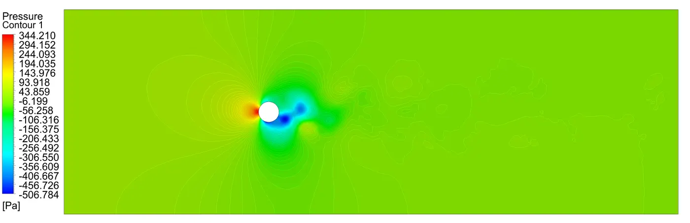
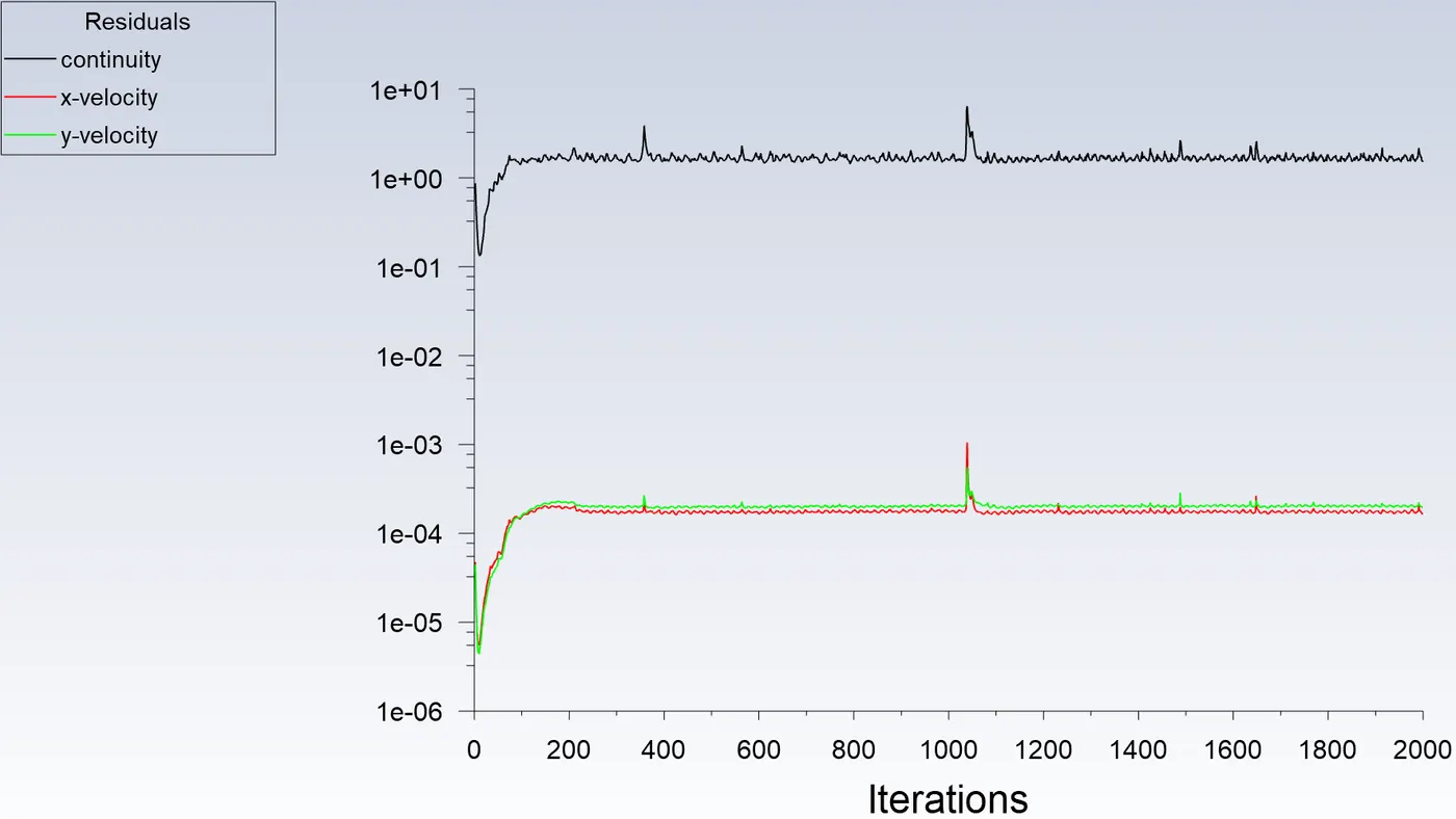
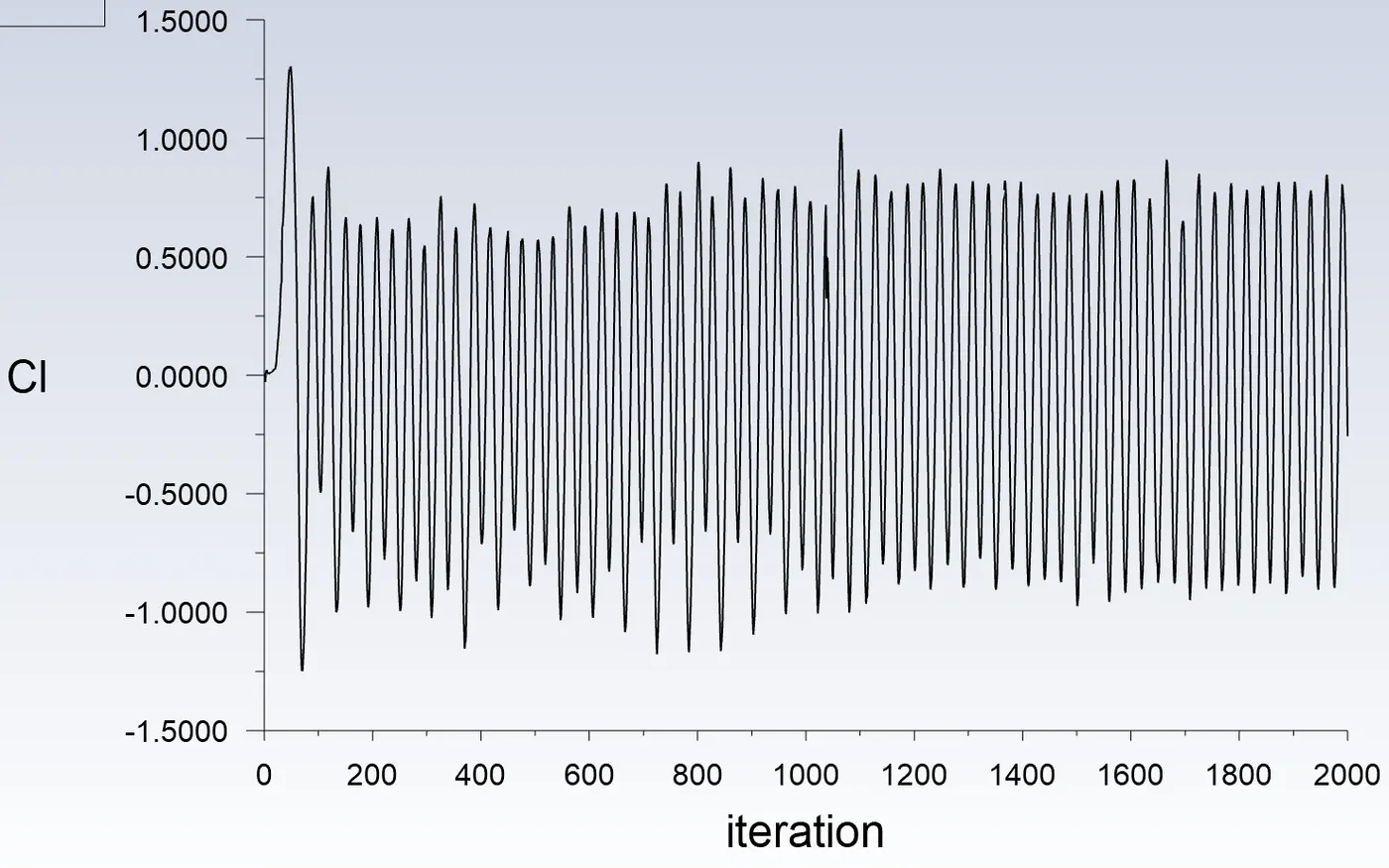
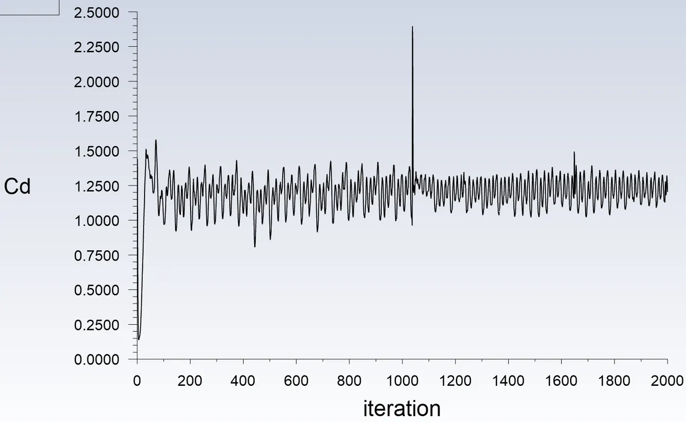
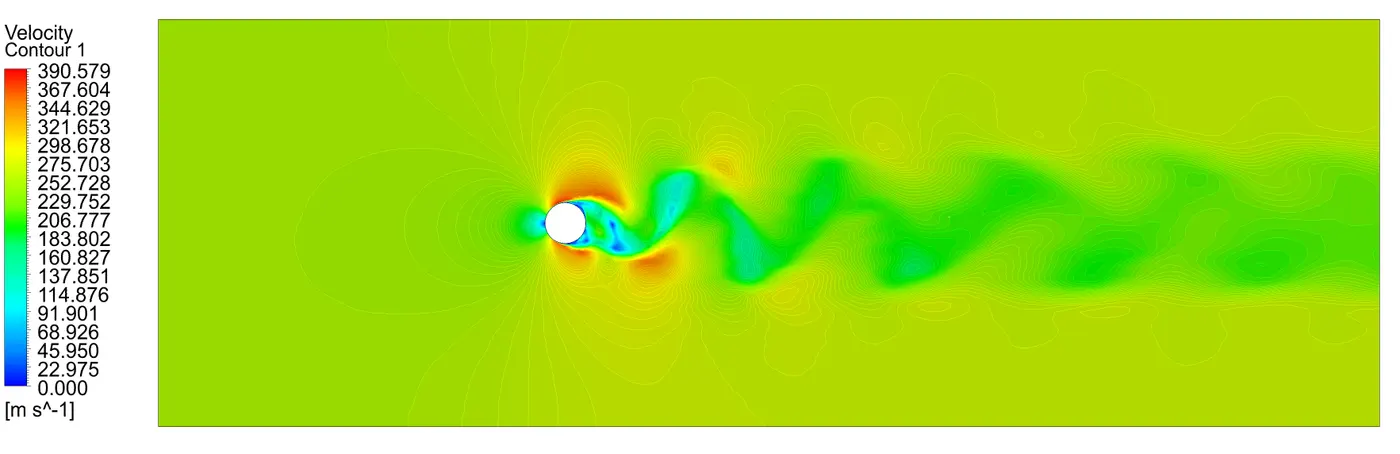
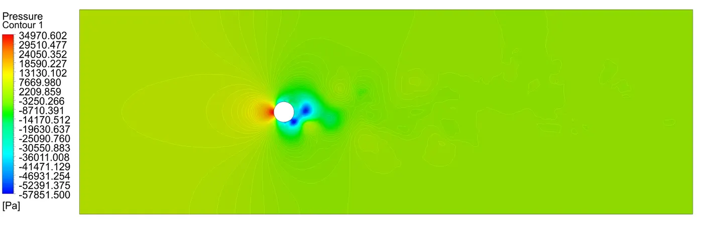
4. Steady State Analysis For Re = 10000 -
Residuals and Solution Monitor Plot -
Contour Plots -
Velocity Contour -
Pressure Contour -
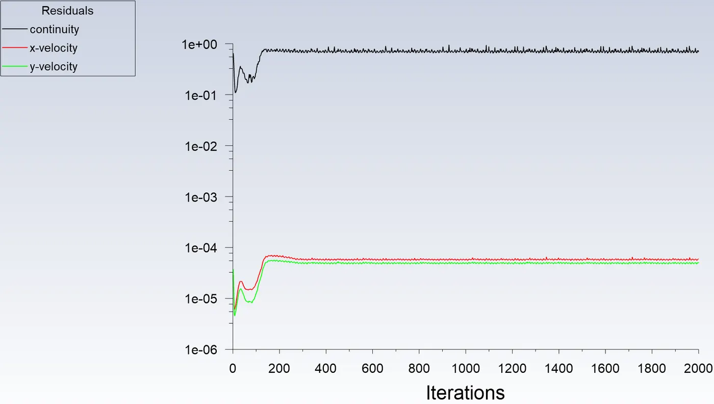
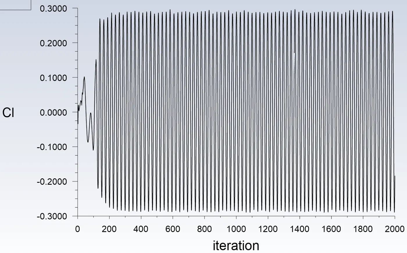
5. Steady State Analysis For Re = 100000 -
Residuals and Solution Monitor Plot -
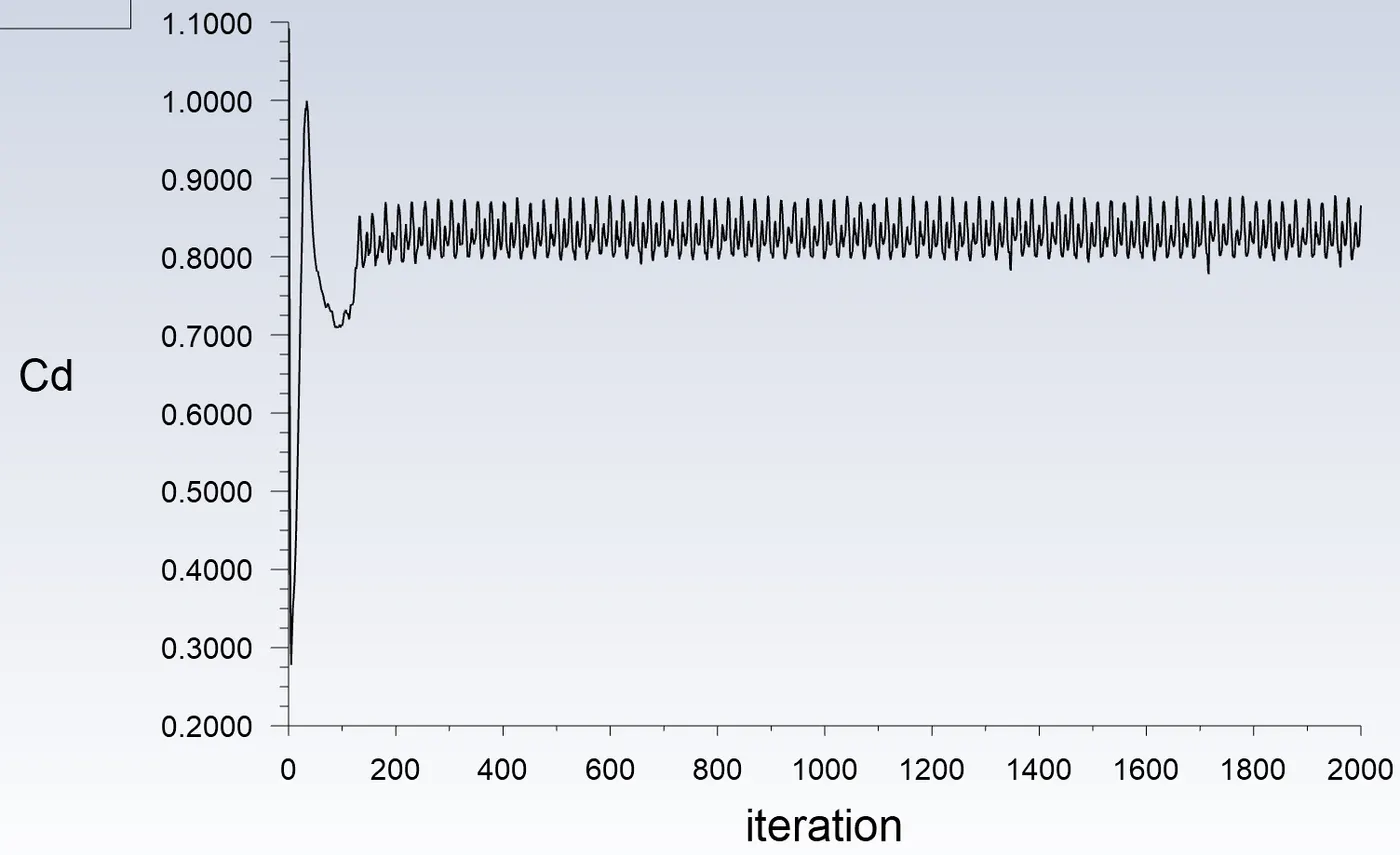
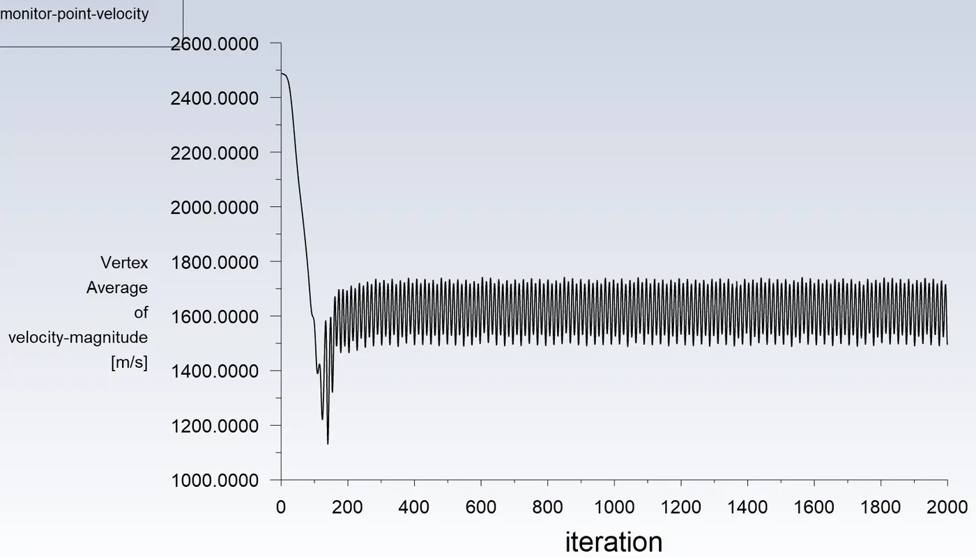
Contour Plots -
Velocity Contour -
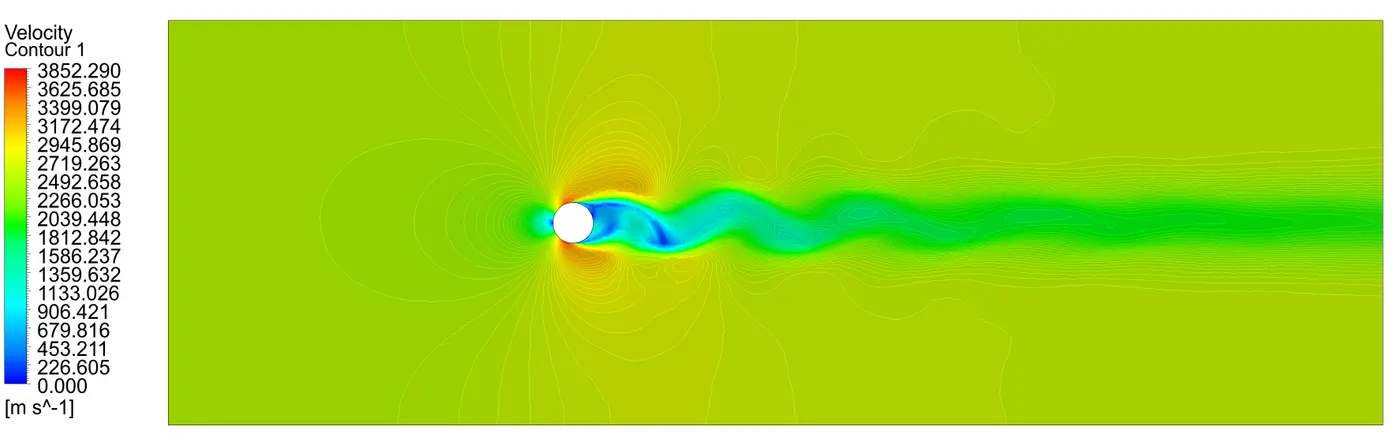
Pressure Contour -
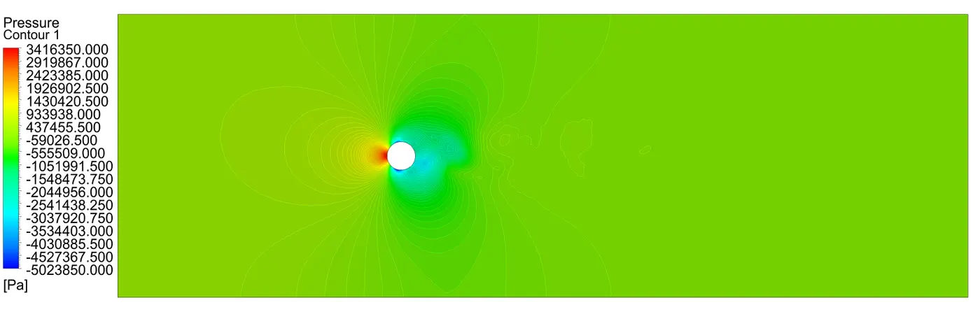
6. Transient Analysis For Re = 10 -
Residuals and Solution Monitor Plot -
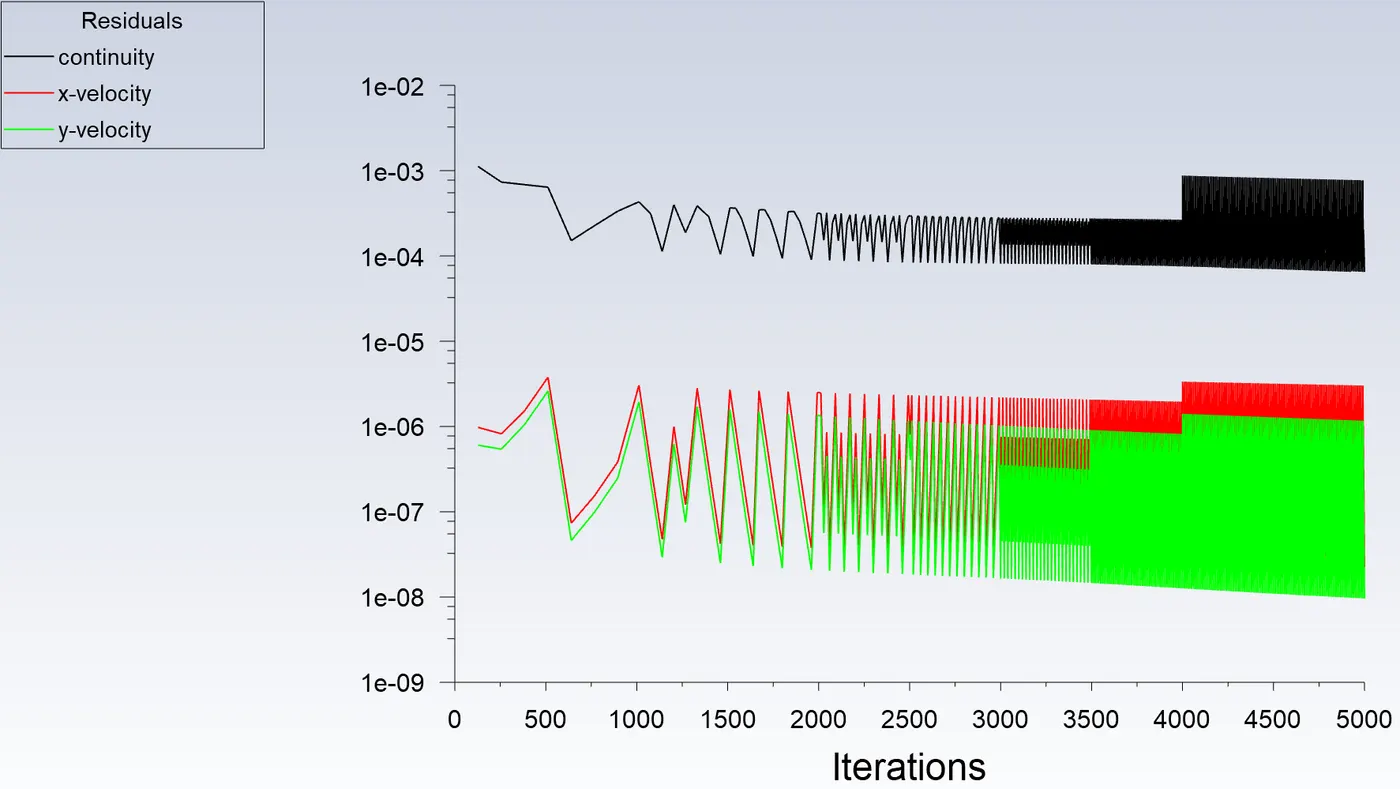
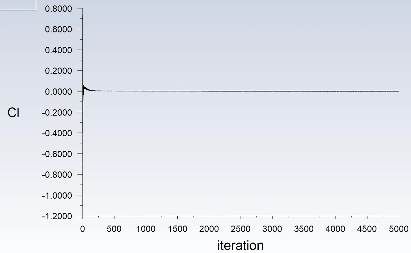
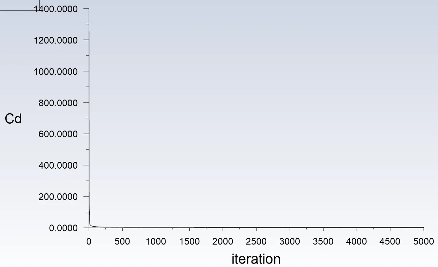
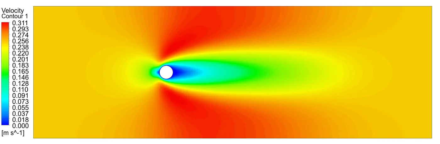
Contour Plots -
Velocity Contour -
Pressure Contour -
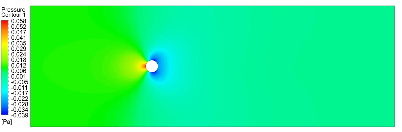
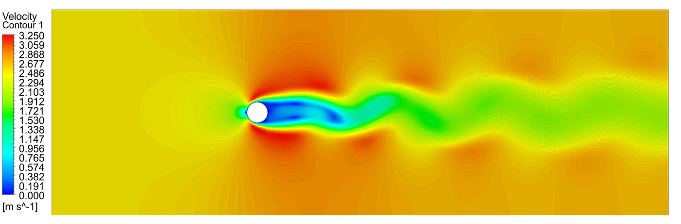
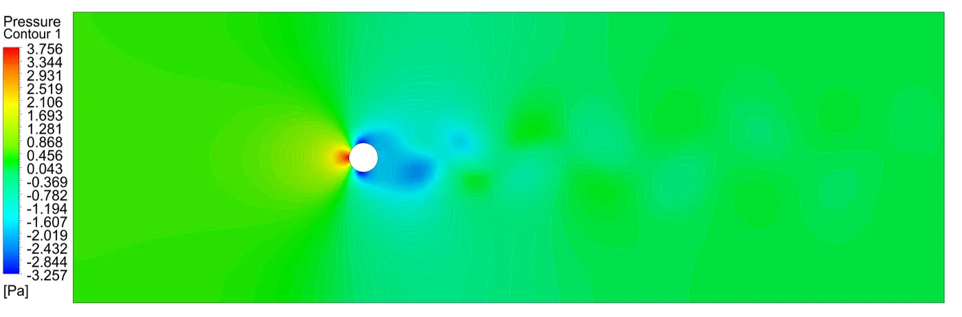
7. Transient Analysis For Re = 100 -
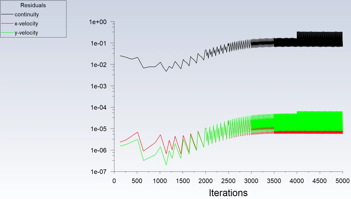
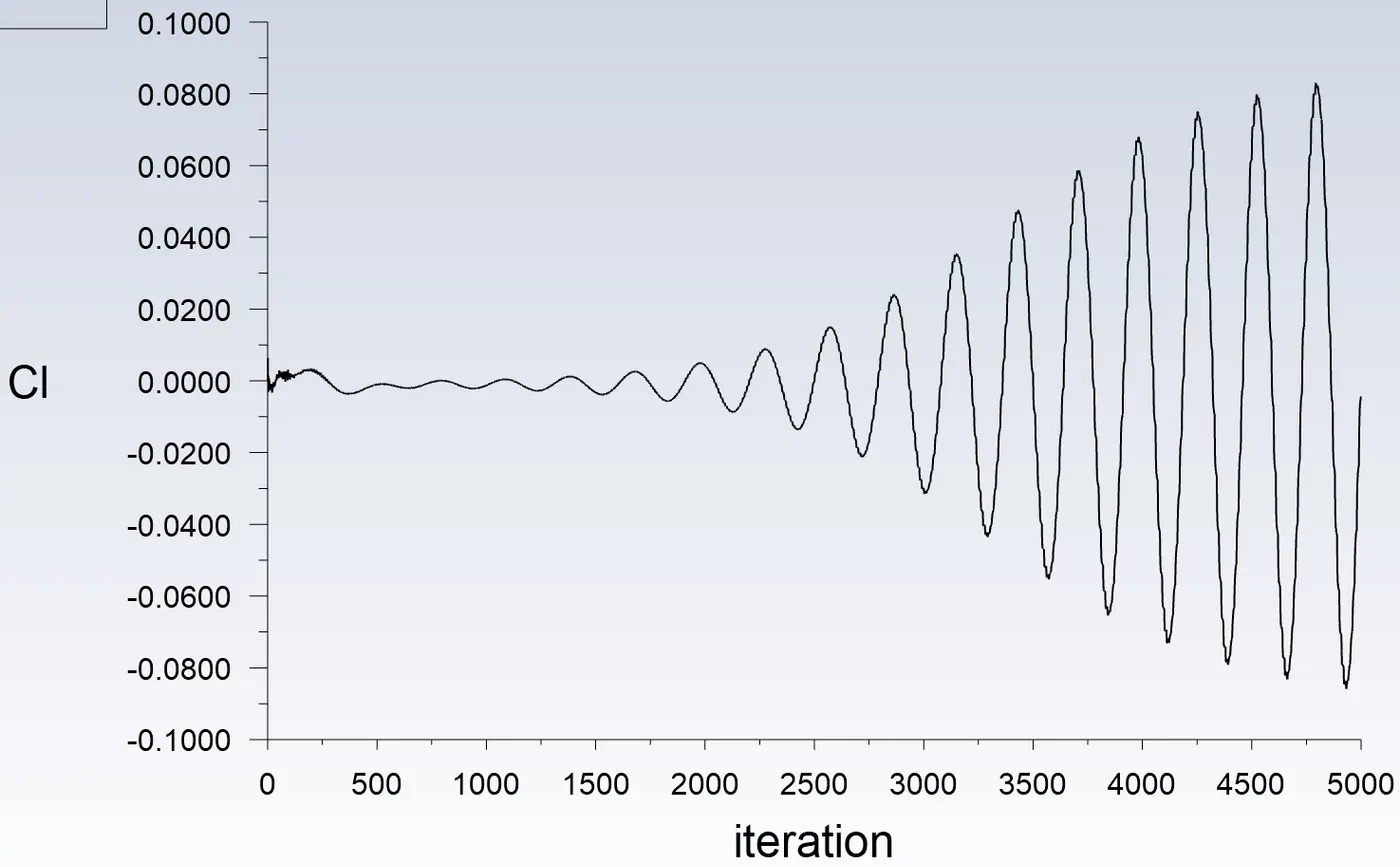
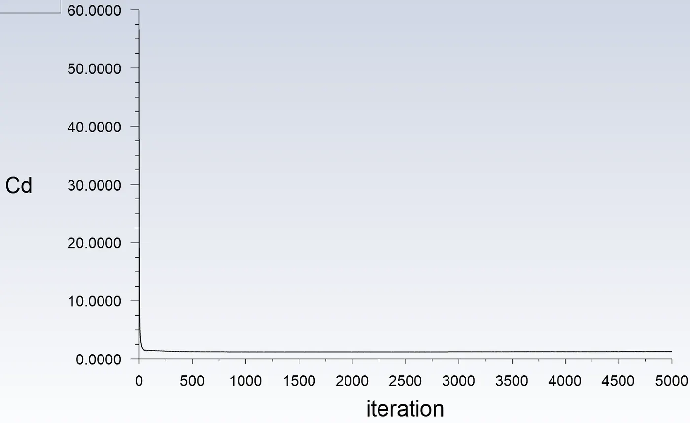
Residuals and Solution Monitor Plot -
Contour Plots -
Velocity Contour -
Pressure Contour -
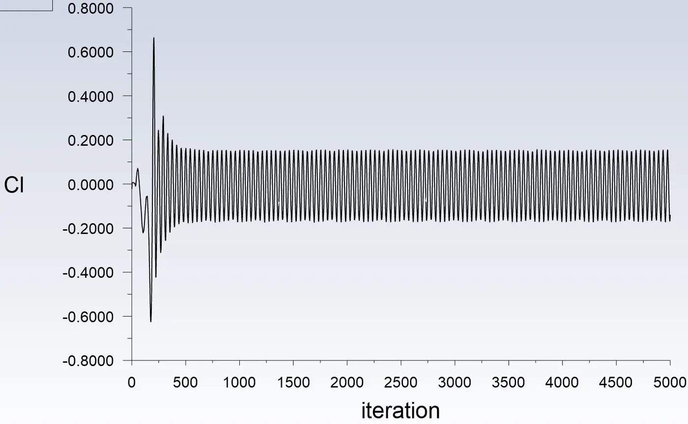
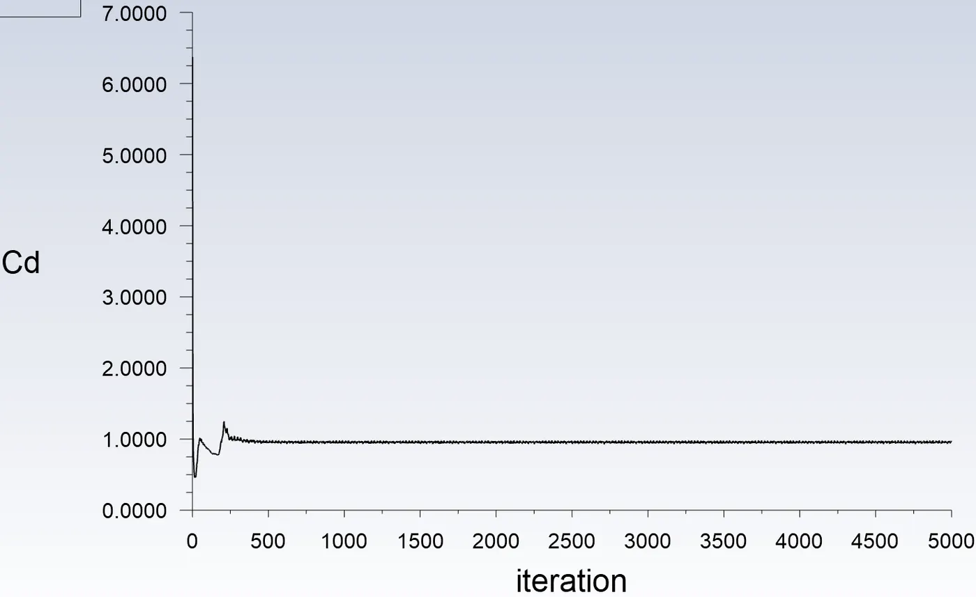
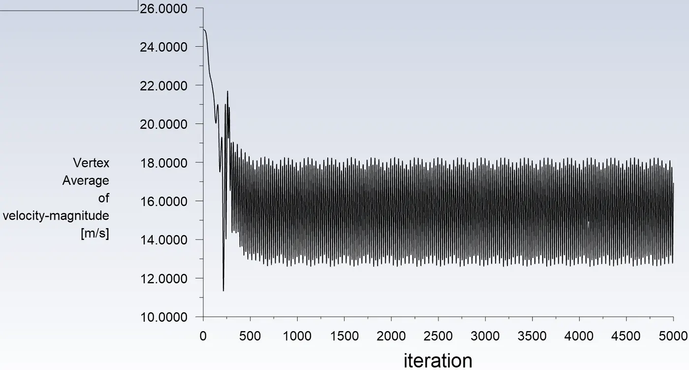
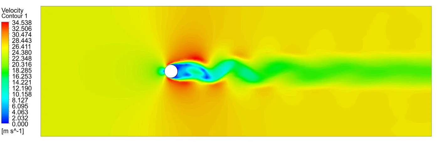
8. Transient Analysis For Re = 1000 -
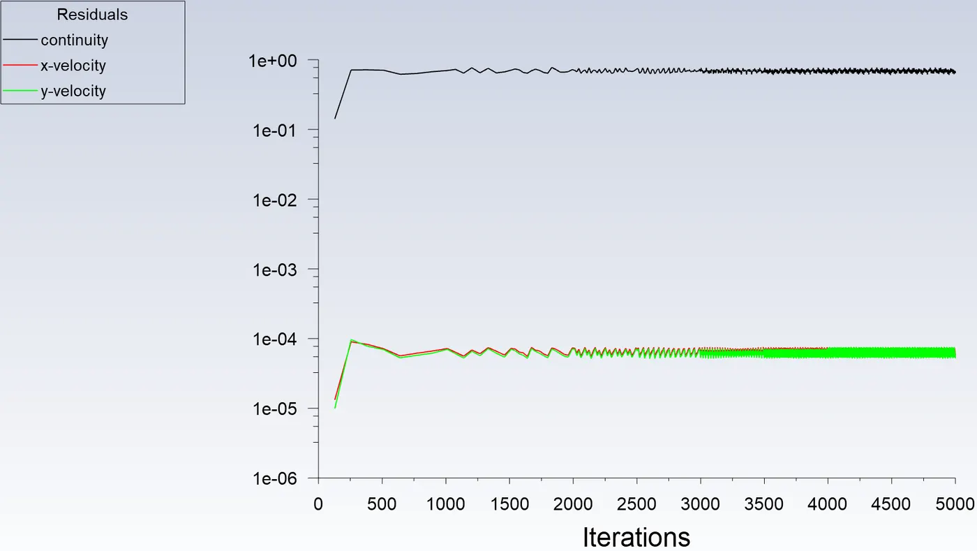
Residuals and Solution Monitor Plot -
Contour Plots -
Velocity Contour -
Pressure Contour -
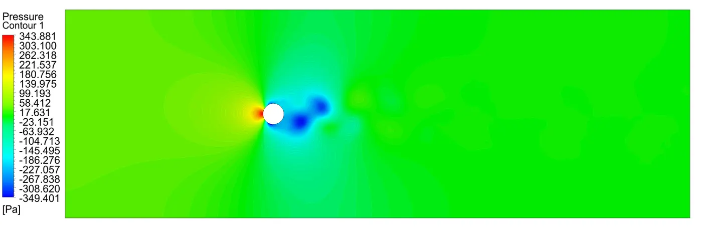
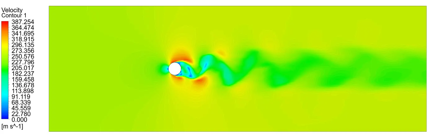
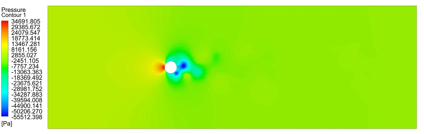
9. Transient Analysis For Re = 10000 -
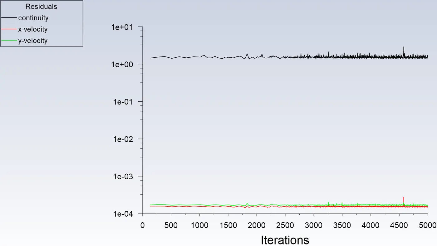
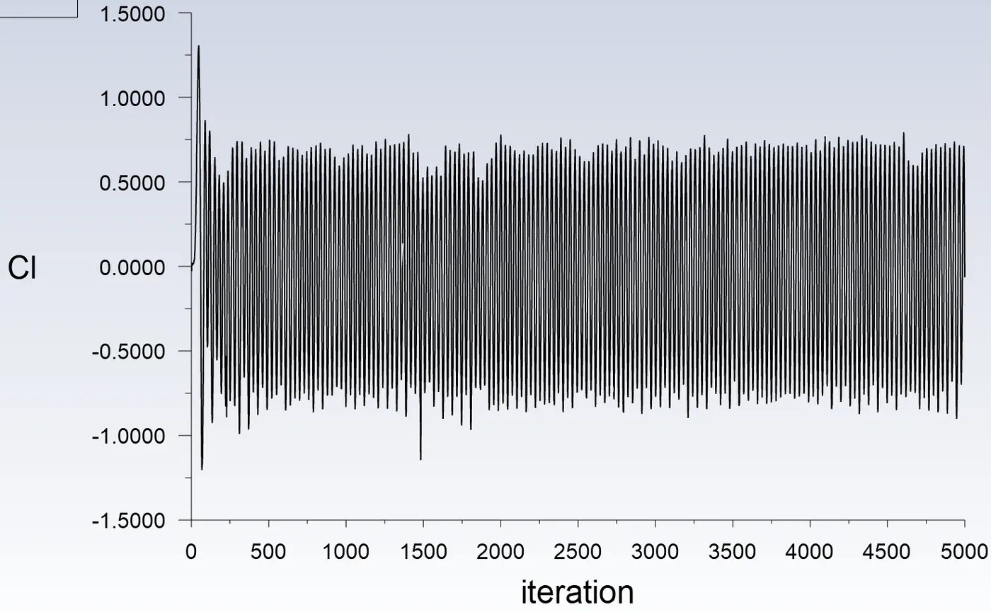
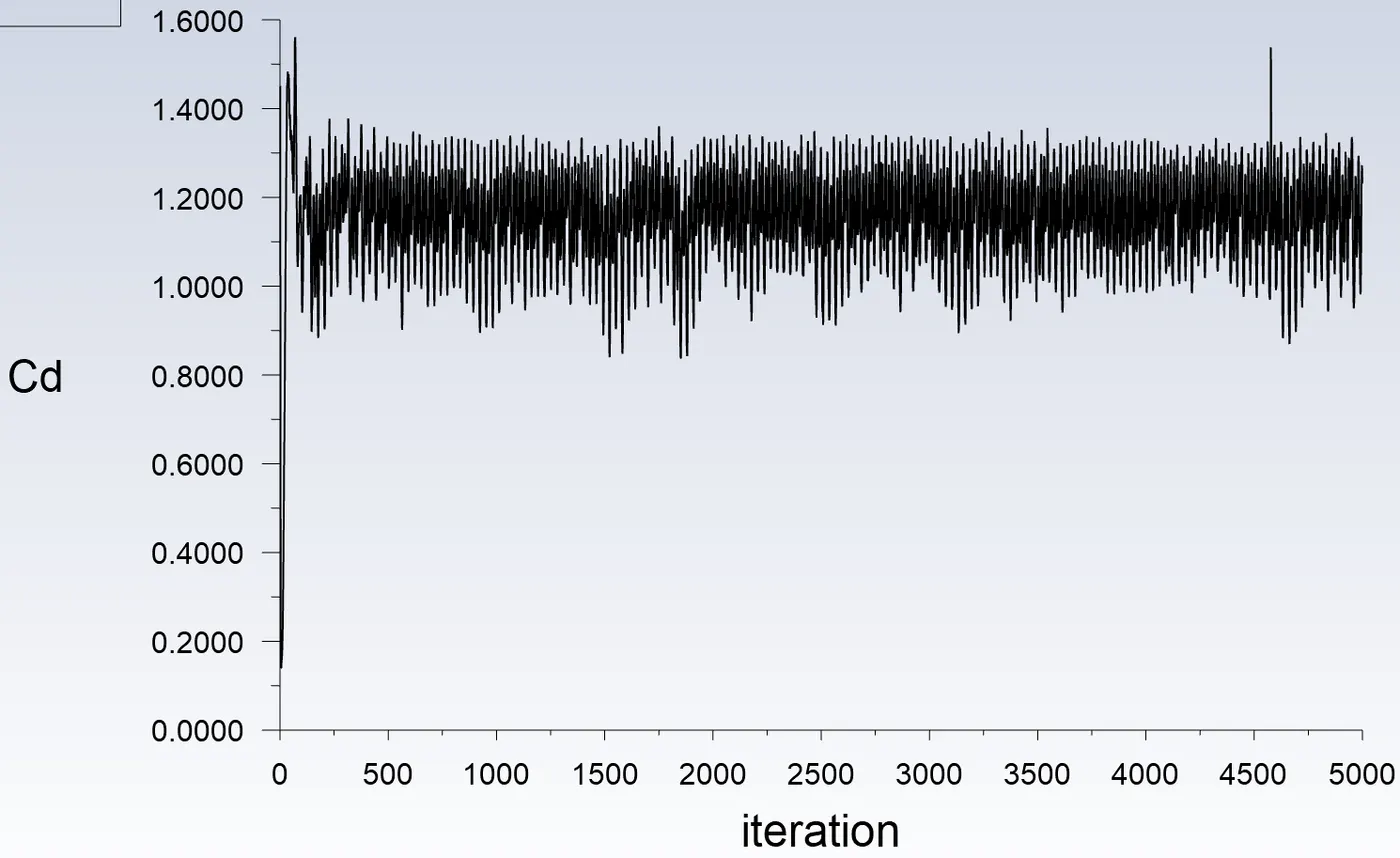
Residuals and Solution Monitor Plot -
Contour Plots -
Velocity Contour -
Pressure Contour -
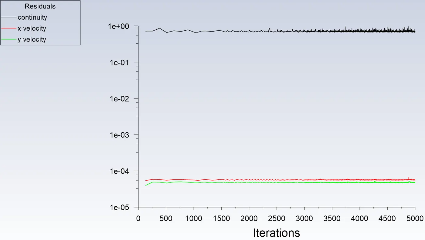
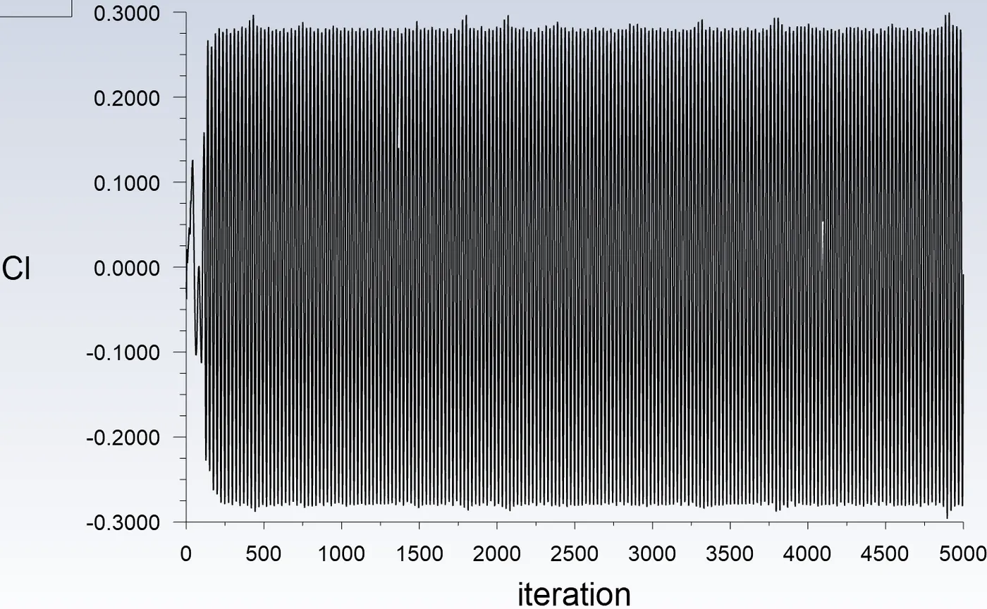
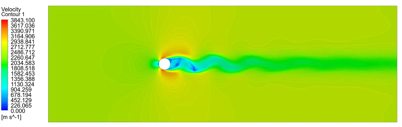
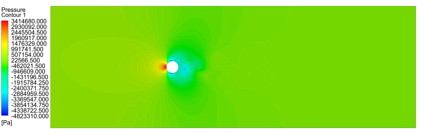
10. Transient Analysis For Re = 100000 -
Residuals and Solution Monitor Plot -
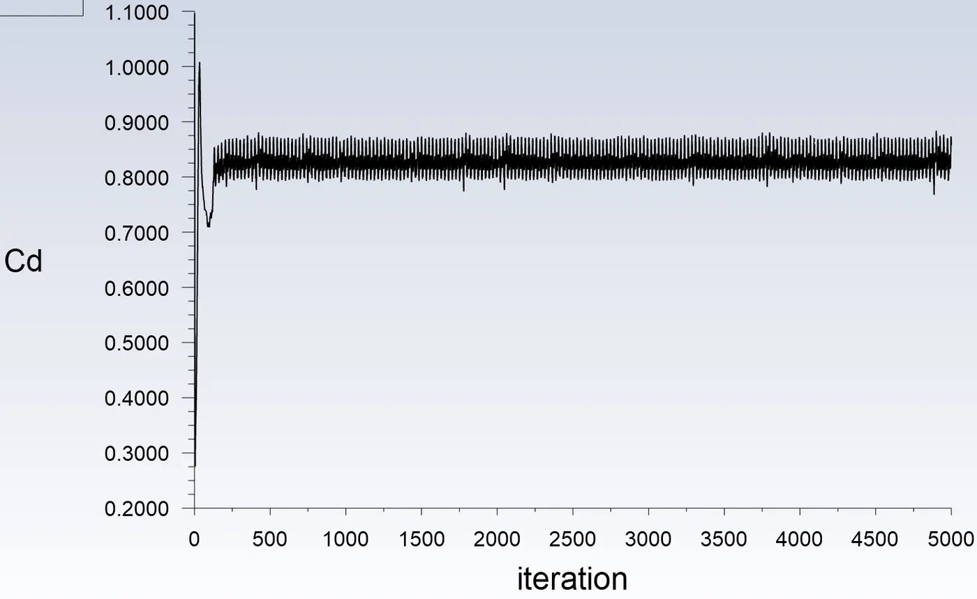
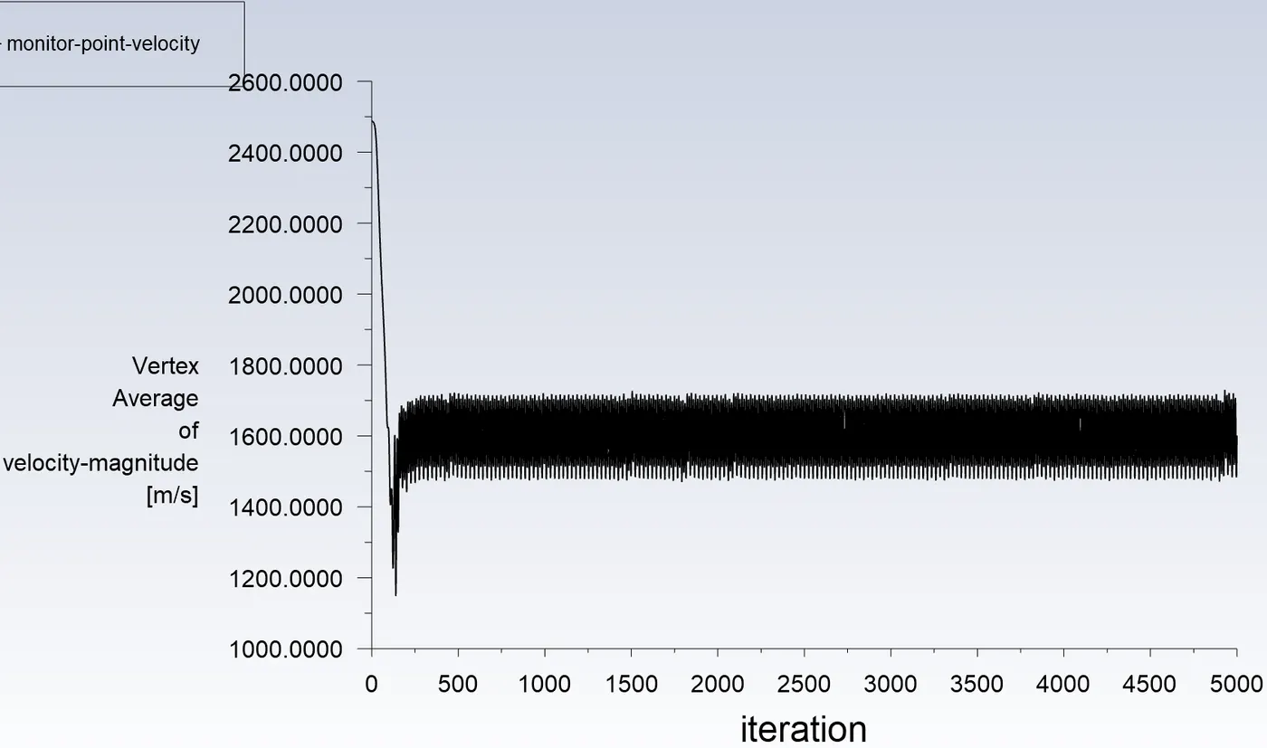
Contour Plots -
Velocity Contour -
Pressure Contour -
RESULTS :
-
Following is the Wind tunnel and experimental data from the research papers,
Taken Reference for the Re 150 ( Ref. [4] )
( Ref. [5] )
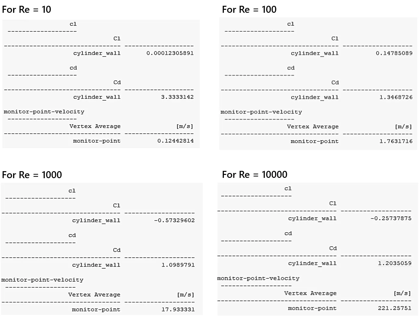
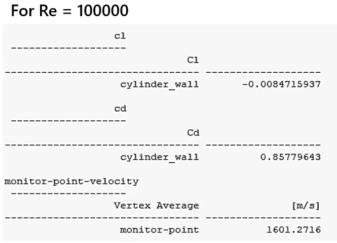
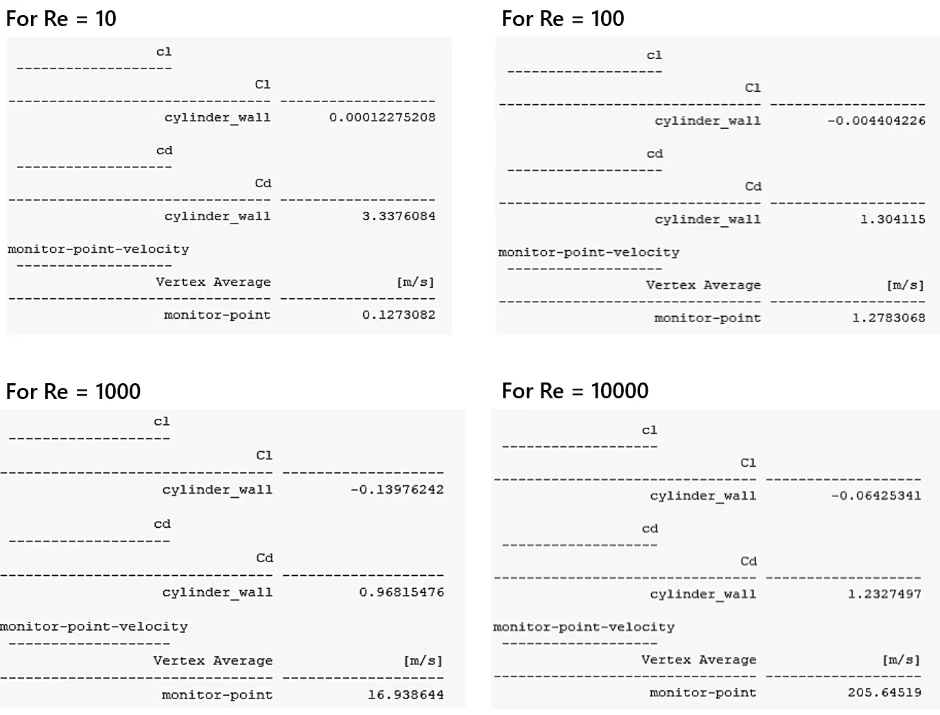
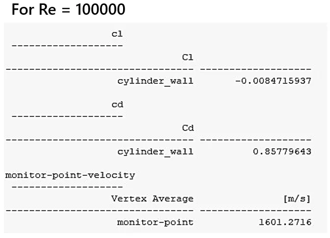
The Following are the summary report of results of the simulation, -
Steady State Simulation -
Transient Simulation -
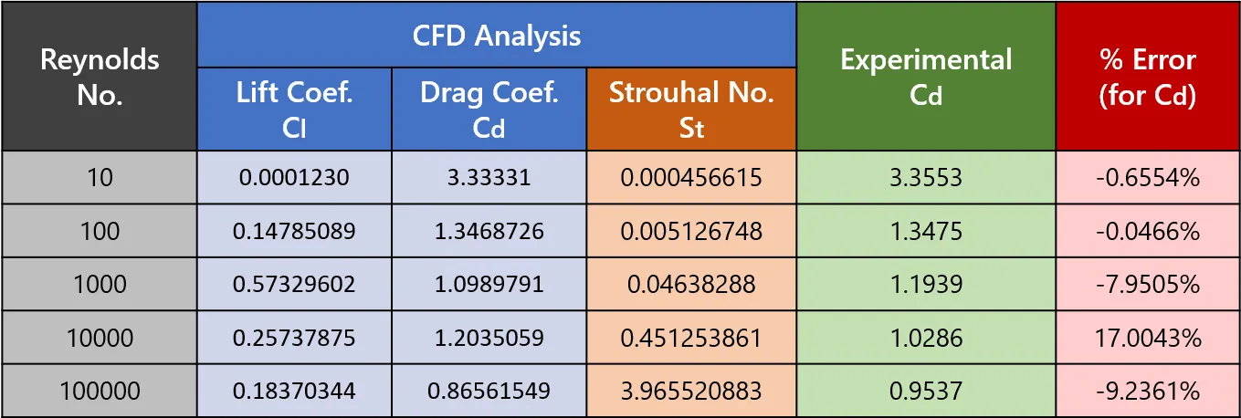
Steady State Analysis -
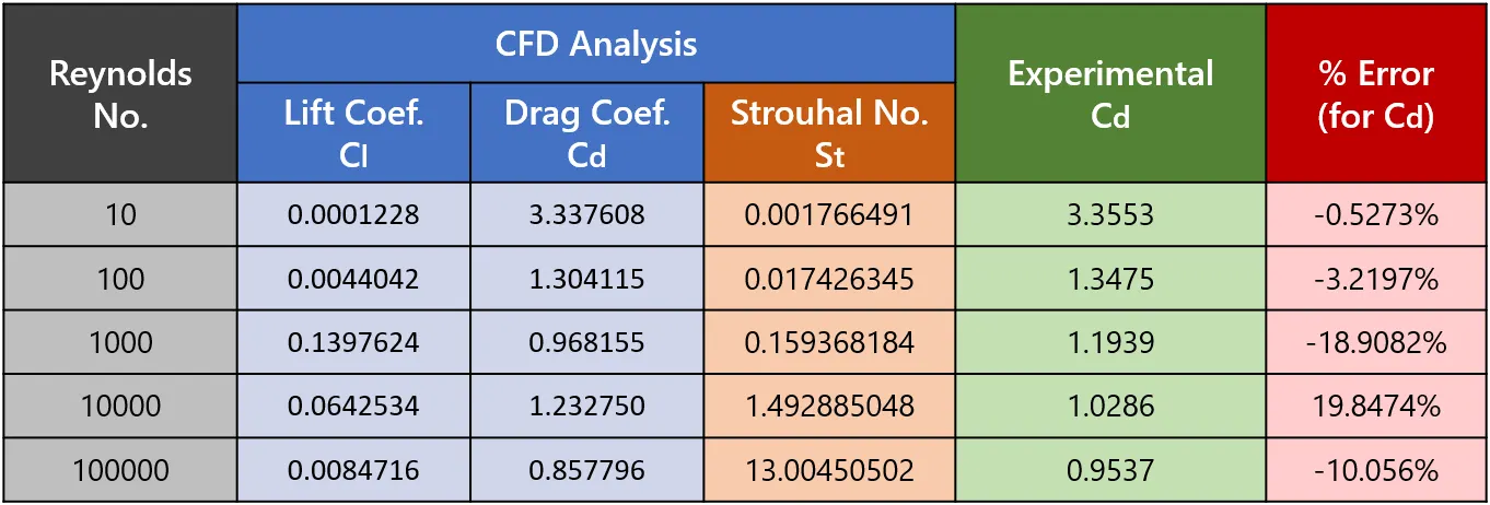
Transient Analysis -
CONCLUSION :
We have successfully performed the analysis of cylinder .
The appropriate Edge Sizing and Inflation were used for optimum Meshing.
The solver was set up using suitable settings to incorporate the physical phenomena.
We were able to generate required contours for speed, & pressure and visualize von karman vortex street.
The following conclusions can be drawn based on the simulation results after running -
- We can see all the residuals are less than 10e-3 for every iteration. Except continuity in the few high velocities.
- The frequency of vortex street increases with increase in Re.
- We can see the drag coefficient decreasing upto Re=10000 after that for the High Re the Drag coefficient increases with the Re.
- Both Steady State and Transient Simulation were completed with all the percentage error less than 20% and for Low Re no. percentage error less than 5%.
For further, inorder for accuracy we can run simulation by more mesh refinement along the walls and using Transition SST Model for transition range or near to transition range reynolds no.
REFERENCE :
- Flow instability and vortex shedding, https://youtu.be/xnr-yRcpnBs
- Vortex shedding and its control | Prof. S. D. Sharma, https://youtu.be/ahohd8ceGR4
- Dynamics and Control of Flow around Circular Cylinder, https://www.youtube.com/watch?v=pW0JfEBE9h8
- John Stack; 'Compressibility Effects in Aeronautical Engineering'; https://ntrs.nasa.gov/citations/20070026133
- NACA TN 3083; Noel K. Delany and Norman E. Sorensen; 'Low-Speed Drag Of Cylinders Of Various Shapes.' https://ntrs.nasa.gov/citations/19930083675
- B.N. Rajani, A. Kandasamy, Sekhar Majumdar; 'Numerical simulation of laminar flow past a circular cylinder' https://www.sciencedirect.com/science/article/pii/S0307904X08000243