Week 6.2 - Setting up a model (Hanging Node)

AIM : To perform Forced convection cooling simulation of the computer enclosure case i.e. created the mesh model for assignment-week 5.2 in Ansys Icepak.

OBJECTIVES :

• Create non-conformal mesh assembly for the components to optimize no. of cells.
• Use multi-level meshing for the required objects.
• Generate mesh & observe in mesh reduction, do visual inspection & check for quality.
• Setup Boundary Conditions, components properties
• Setup solver Settings and monitor points
• Getting results & Post-Processing

INTRODUCTION :

Components are often designed to generate as little heat as possible, and computers and operating systems may be designed to reduce power consumption and consequent heating according to workload.

Electronic cooling is required to remove the waste heat produced by computer components, to keep components within permissible operating temperature limits. Components that are susceptible to temporary malfunction or permanent failure if overheated include integrated circuits such as central processing units(CPUs), chipset, graphics cards, and hard disk drives.

Multi-Level meshing is the tool available in Ansys Icepak which is used to mesh and capture complex CAD geometry. Multi-level meshing tool allows to set levels to different components and zones in the geometry setup. For the regions where CAD is very important or CAD is very complex there the mesh will be very dense and where there is less complex geometry or less important area there will be coarse mesh.

The level of multi level mesh goes as follows -

• 0th Level - the mesh cell is the gneral coarse initial mesh cell size.
• 1st Level - will be 4 cells equal-divides of the previous cell.
• 2nd level - will be again each 1st level cell is divided into 4 parts.

like that at every level the each previous cell is divided into 4 equal parts.

STEPS / PROCEDURE :

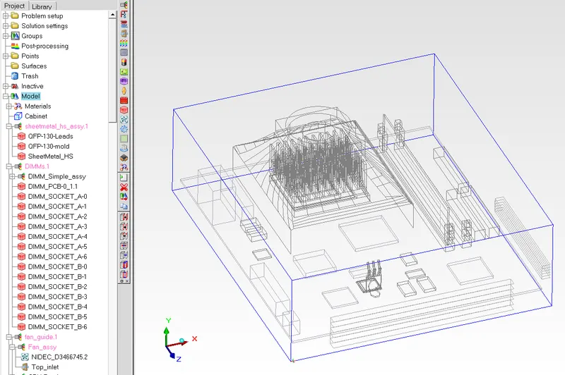
1) Loading Geometry/the given case setup from the project file.

Following are the Geometry of the given Case -

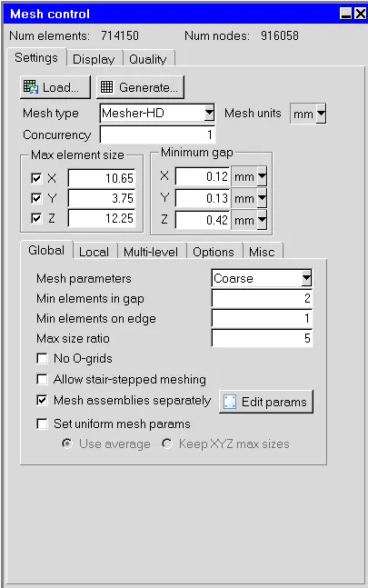
2) Generating Preliminary coarse mesh on the gemotry as it is.

Following the mesh size of the generated mesh -

3) Creating Mesh assembly and non-conformal meshing for optimizing the mesh count for the simulation case.

Following is the mesh assemblies created and non-conformal meshing mesh count -

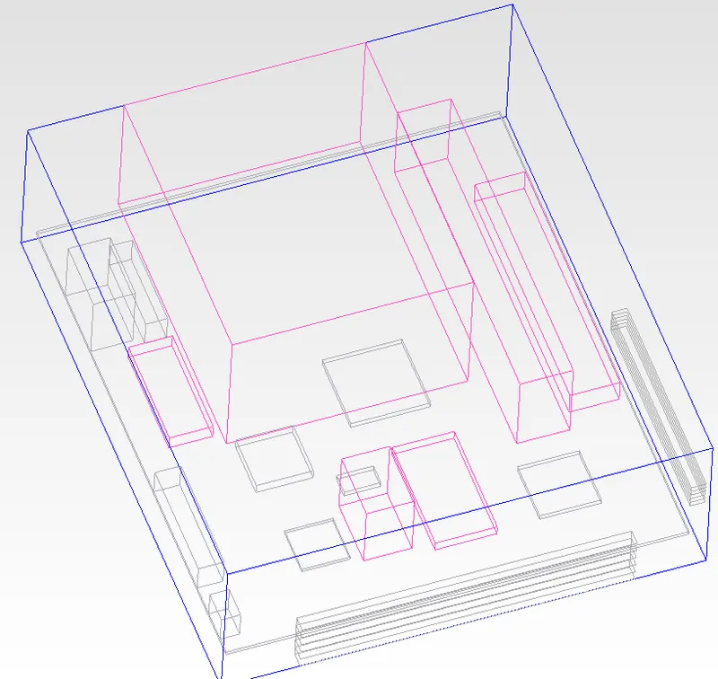
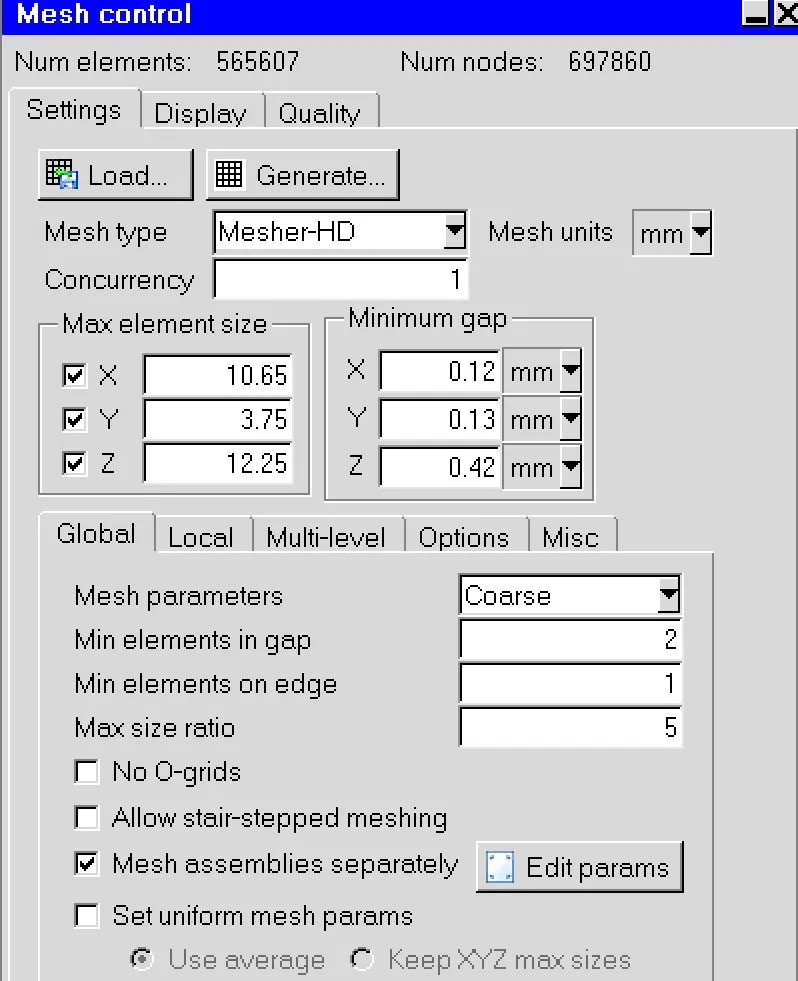
We can see that there is very significant decrease in the mesh count compared to previous generated mesh.

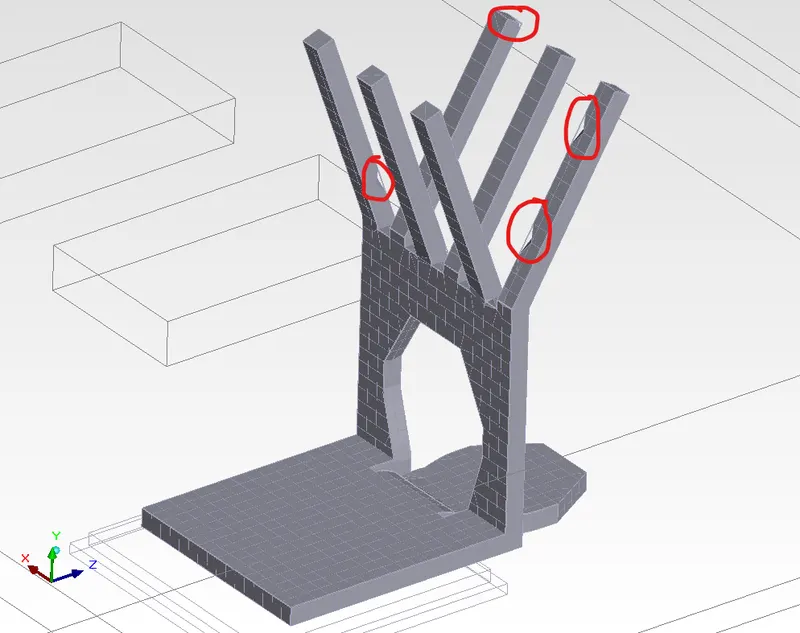
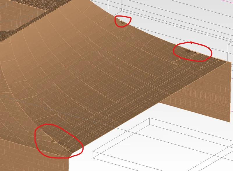
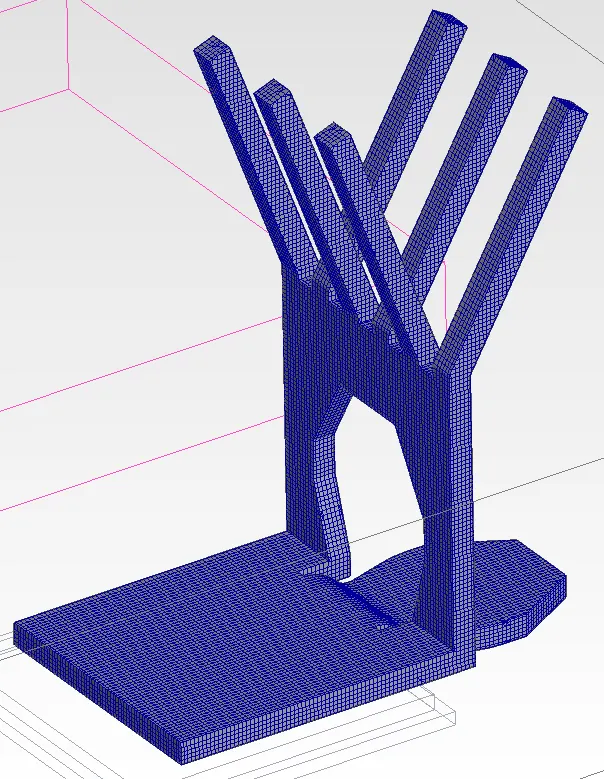
3) But we when inspect the mesh we can see that there are some irregularties in regions of the complex geometry gemotry components where mesh is not nicely and formed and not capture the component correctly. Examples of two components are shown below, -

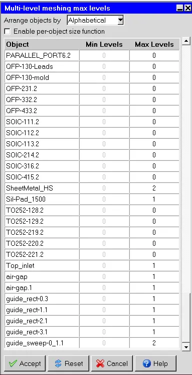
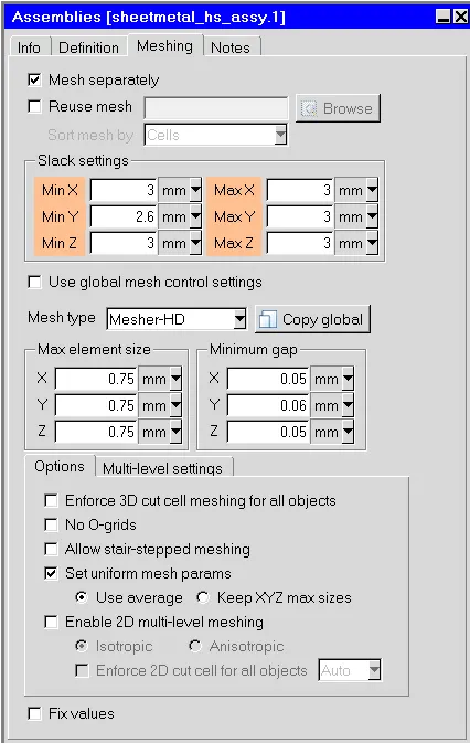
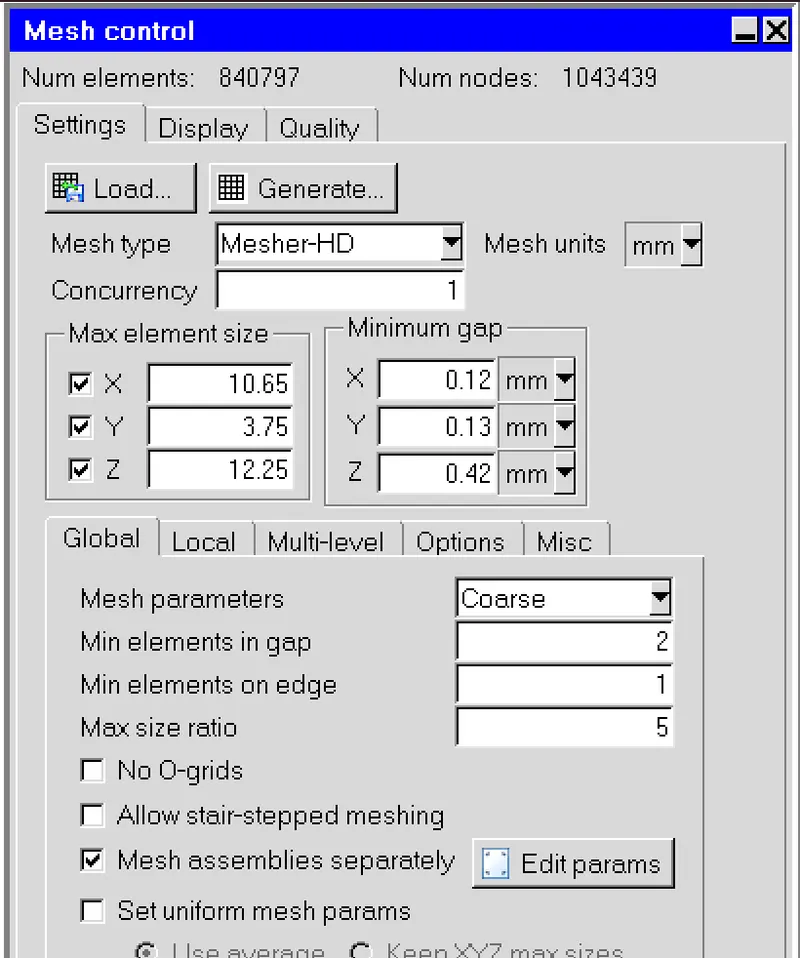
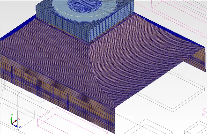
4) So Multi Level Meshing tool is being to make finer mesh to these components specifically with relative to other components and nearby regions.

Along with this setting we can also use set uniform mesh parameter with average setting, which will create uniform mesh cells on the region by averaging.

5) Mesh Quality Parameters

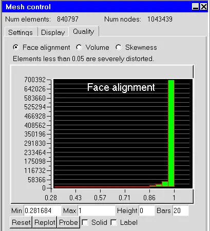
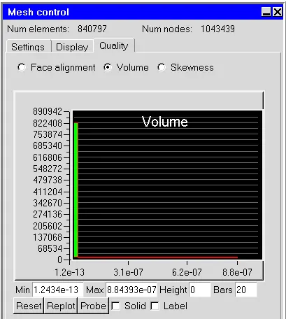
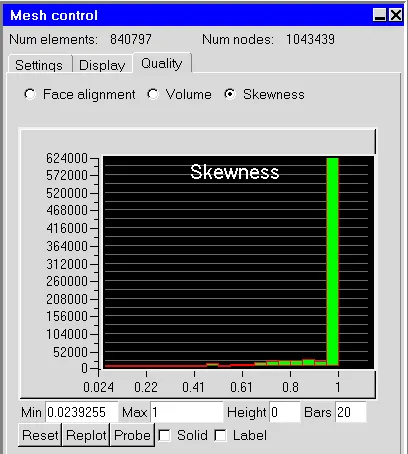
We can the mesh quality is very satisfied. 90% of the mesh cell are lying on good quality range.

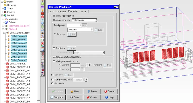
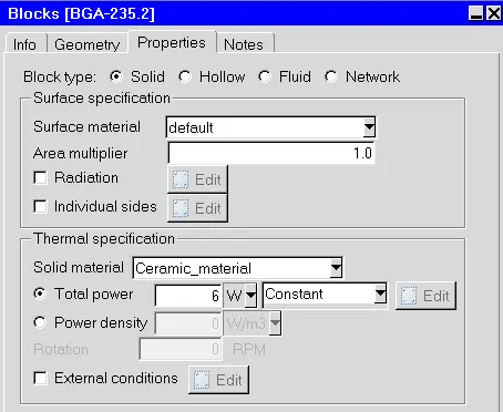
6) Component Properties & Settings -

Sources and their properties -

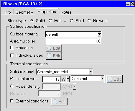
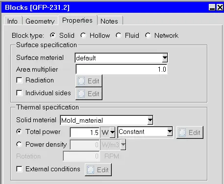
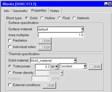
Fan and Flow Properties -

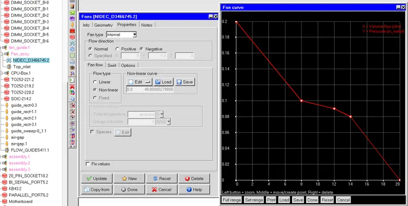
7) Solver Settings -

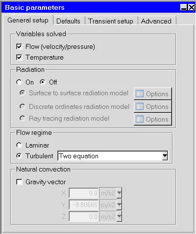
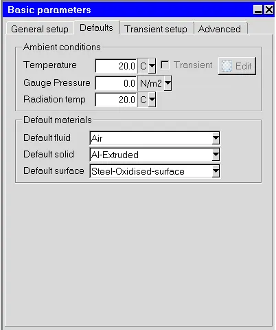
Gravity option is turned off since the majority of the fluid flow is affected by the fan i.e. force convection compared to natural convection.

Inorder to capture the turbulence flow conditions we have chosen two equation model option i.e. K-epsilon turbulaance model. Since in the forced convection vortices / turbluence plays major roll in the heat transfer and therefore cooling.

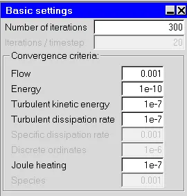
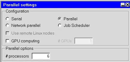
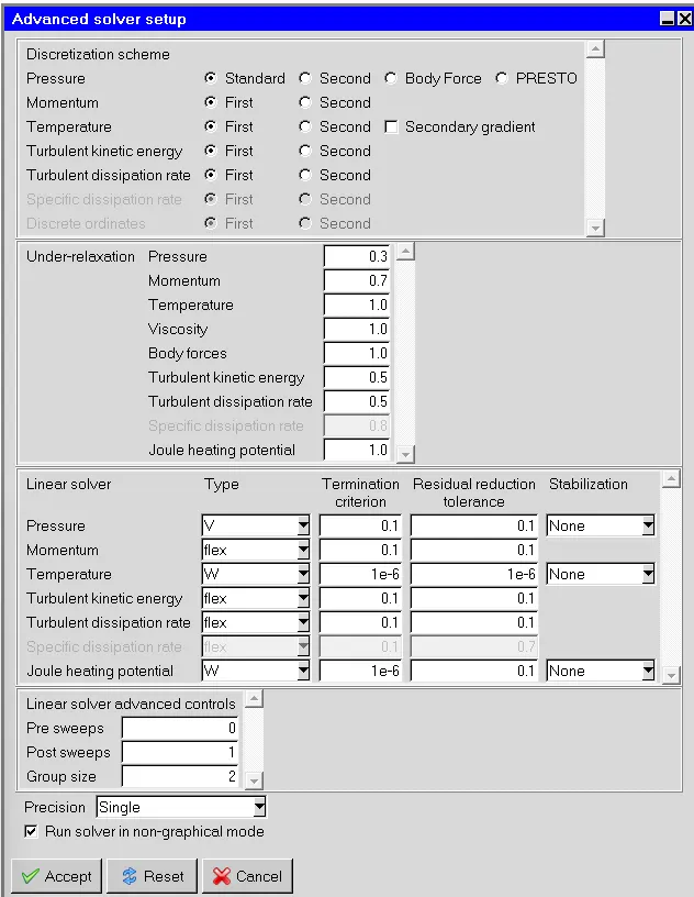
The solver setting majorily have kept default. and the discretization schemes are kept 1st order in-order to get stable first cut simulation.

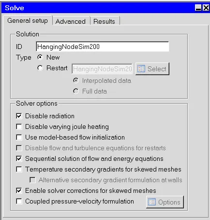
Radiation solver has been disabled because majority of heat transfer is happening through forced convection.

We have selected here sequential solution of flow and energy equation, which is simply that the solver will first solve the flow equations to define the flow and then the energy equations are solved for the temperature.

POST PROCESSING :

Outputs

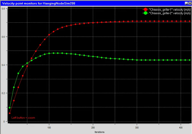
Residuals and Monitor Points -

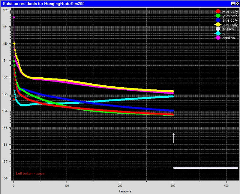
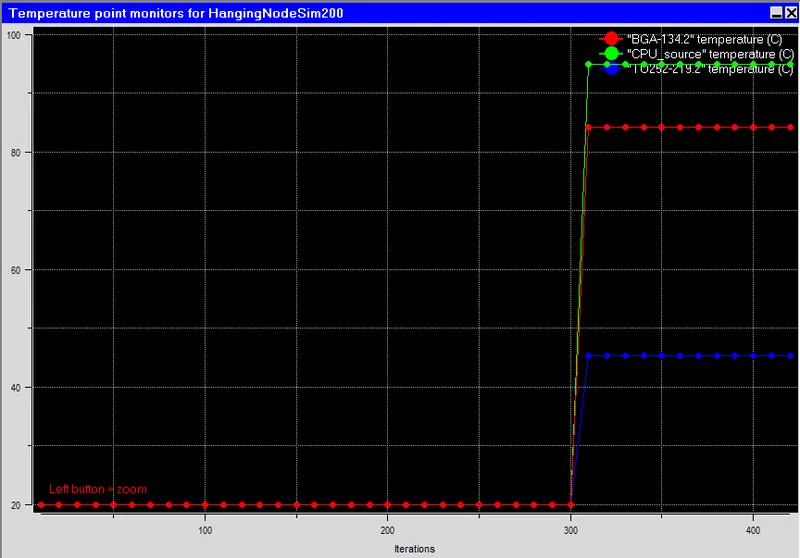
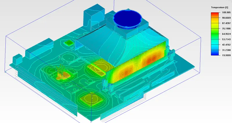
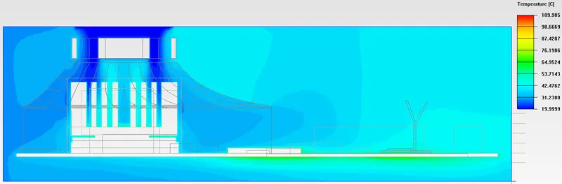
Temperature Contours -

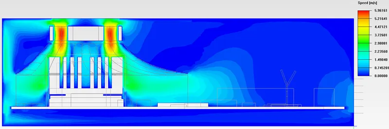
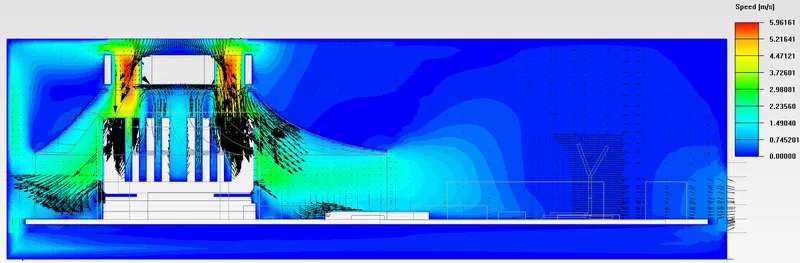
Contour and Streamline Visulization of Velocity of the fluid -

RESULTS :

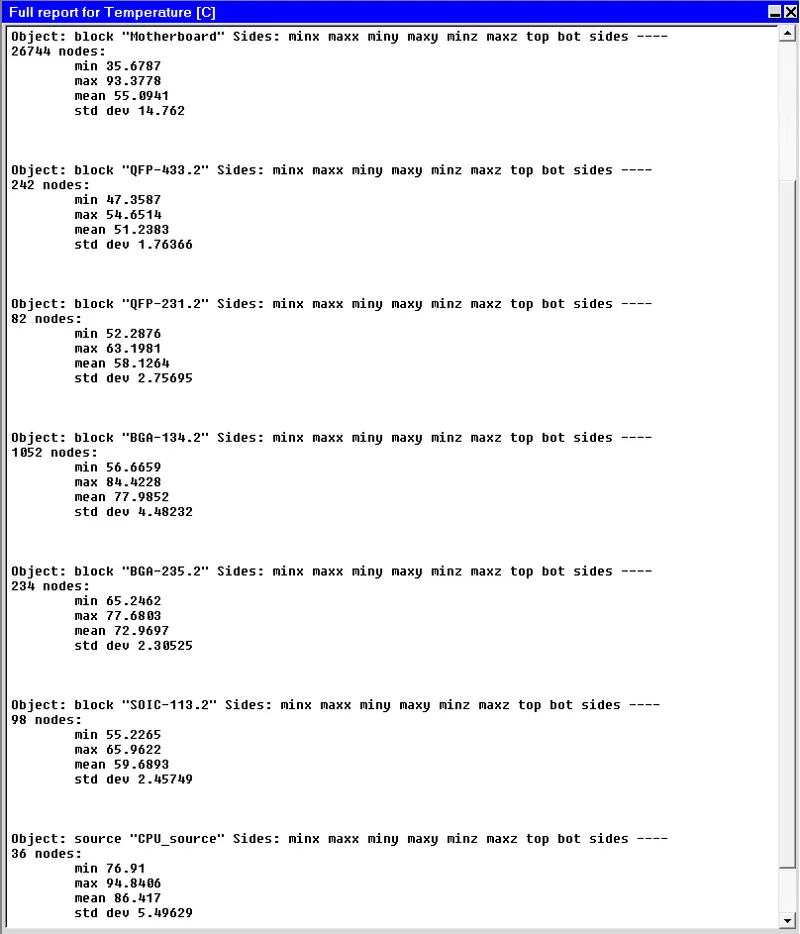
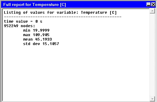
The Following are the results of the simulation, generated simulation report from the ICEPAK software Showing Various characteristic values of the simulation and the max. temperatures of the different bodies acting in the simulation -

CONCLUSION :

We have successfully performed the simulation analysis for a hanging node model and obtained the results by post-processing. And separately meshed assemblies have been employed to reduce the overall mesh count in the domain.

Parameters like temperature and velocity were plotted. And monitor points were considered at the plates and blocks to obtain the temperature and velocity that has generated in the model.

From the results we got 109 Celsius maximum temperature is observed at the DIMMs. The operating temperature of electronics components have generally have critical temp. of 115-120 degrees, the maximum temperature is coming 109 but temperatures above 100 degree decrease life expentancy of components. So either to make more fine mesh simulation and verifying the accuracy of the first cut simulation and then make changes in the design to improve thermal management of the system.