Week 5 - Rayleigh Taylor Instability

AIM : To perform the Rayleigh Taylor instability simulation for two dimensional multiphase flow of two immiscible fluids.

OBJECTIVES :

• Setting up the Geometry in Spaceclaim.
• Create optimal meshing for the model in Ansys Mesher.
• Setup the model for the analysis from the given data.
• Run the simulation and Post Process the results.
• Capturing the Rayleigh Taylor instability between the two immiscible fluids and calculate the Atwood number for them.
• Run the simulation for 3 mesh levels.
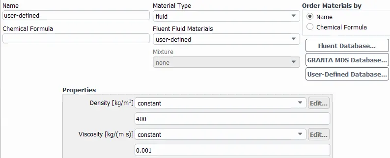
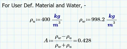
• Also check for both 1) water and air and 2) water and user defined fluid (with Density of 400 Kg/m3 and Viscosity 0.001 Kg/ms).

INTRODUCTION :

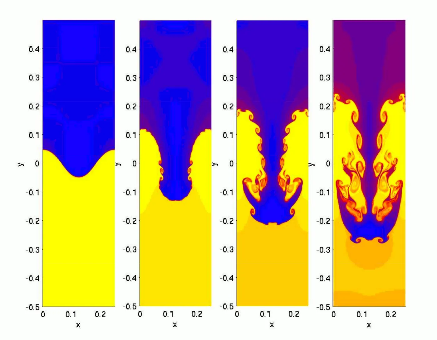
Rayleigh–Taylor instability or RT instability is the instability of an interface between two fluids of different densities which occurs when the lighter fluid is pushing the heavier fluid. As the RT instability develops, the initial perturbations progress from a linear growth phase into a non-linear growth phase, eventually developing "plumes" flowing upwards (in the gravitational buoyancy sense) and "spikes" falling downwards. In the linear phase, the fluid movement can be closely approximated by linearly, and the amplitude of perturbations is growing exponentially with time. In the non-linear phase, perturbation amplitude is too large for a linear approximation, and non linearity is required to describe fluid motions.

(Source: Wikipedia)

Atwood Number

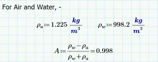
It is a dimensionless number which is defined as the ratio of the difference between the heavier fluid density and the lighter fluid density to their sum. It used in the study of hydrodynamic instabilities in density stratified flows. It is an important parameter in the study of Rayleigh-Taylor instability and Richtmyer-Meshkov instability.

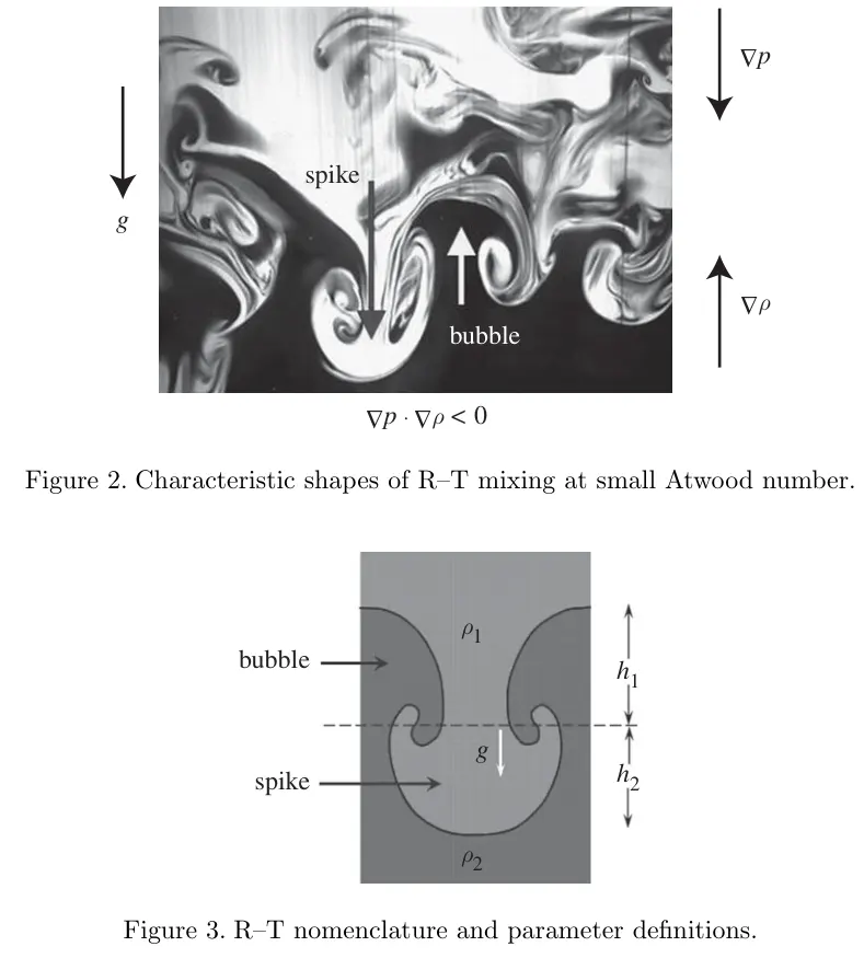
In Rayleigh–Taylor instability, the penetration distance of heavy fluid bubbles into the light fluid is a function of acceleration time scale. In essence, the Atwood number provides valuable insights into the behavior of fluids with different densities when they interact, making it a crucial tool in fluid dynamics.

`A=(rho_1-rho_2)/(rho_1+rho_2)`

where,

ρ1= density of heavier fluid

ρ2= density of lighter fluid

For A close to 0, RT instability flows take the form of symmetric "fingers" of fluid; for A close to 1, the much lighter fluid "below" the heavier fluid takes the form of larger bubble-like plumes.

( Ref - [3] )

Different types of Instabilities

1) Richtmyer–Meshkov instability

The Richtmyer–Meshkov instability (RMI) occurs when two fluids of different density are impulsively accelerated. Normally this is by the passage of a shove wave. The development of the instability begins with small amplitude perturbations which initially grow linearly with time. This instability can be considered the impulsive-acceleration limit of the Rayleigh-Taylor Instability

2) Kelvin Helmholtz indtability

The Kelvin–Helmholtz instability can occur when there is velocity shear in a single continuous fluid or where there is a velocity difference across the interface between two fluids. An example is wind blowing over water.

3) Plateau Rayleigh instability

The Plateau–Rayleigh instability, often just called the Rayleigh instability, explains why and how a falling stream of fluid breaks up into smaller packets with the same volume but less surface area. It is related to the Rayleigh-Taylor Instability and is part of a greater branch of fluid dynamics concerned with fluid thread breakup. This fluid instability is exploited in the design of a particular type of ink jet technology whereby a jet of liquid is perturbed into a steady stream of droplets. The driving force of the Plateau–Rayleigh instability is that liquids, by virtue of their surface tension, tend to minimize their surface area.

4) Staffman Taylor instability

The Saffman–Taylor instability, also known as viscous fingering, is the formation of patterns in a morphologically unstable interface between two fluids in a porous medium. This situation is most often encountered during drainage processes through media such as soils. It occurs when a less viscous fluid is injected, displacing a more viscous fluid.

CFD model based on mathematical analysis of RT instability

1) Volume of Fluid (VOF)

In CFD, the volume of fluid (VOF) method is a free surface modeling technique for tracking and locating the free surface or fluid - fluid surface. It belongs to the class of Eulerian methods which are characterized by a mesh that is either stationary or is moving in a certain prescribed manner to accommodate the evolving shape of the interface

2) K-L turbulence model

The K-L model was proposed by Dimonte and Tipton for describing the turbulent self-similar regime of RT and RM induced mixing. The model describes the dominant eddies in the mixing zone with evolutionary equations for their characteristic dimension (L) and energy per unit mass (K).

3) Kelvin-Helmholtz / Rayleigh Taylor Hybrid Model

This model was used to predict the primary break up of the intact liquid core of the jet and the Raleigh Taylor model determines the effects of acceleration of the different phases. This model predicts the shape of the spray considering the temperature at different phaces.

STEPS / PROCEDURE :

1) Geometry

The Following is the geometry based on given data in spaceclaim -

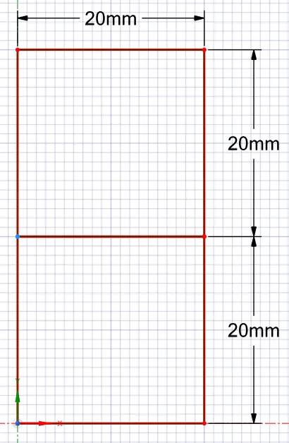
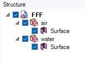
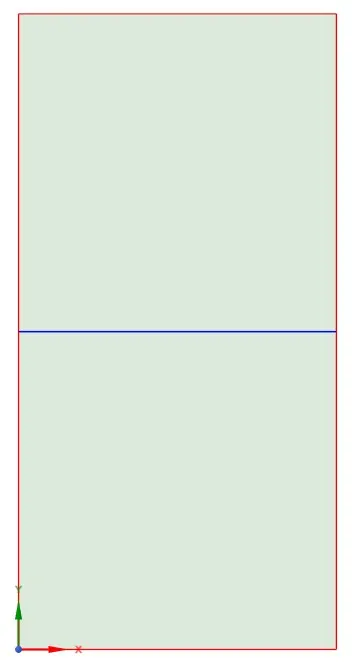
Make sure to enable share topology

2) Meshing

After doing Geometry preparation, we gone open the geometry in Ansys Mesher via workbench -

• Creating Named Selections
• Assigning proper mesh sizing
• Checkng mesh quality.

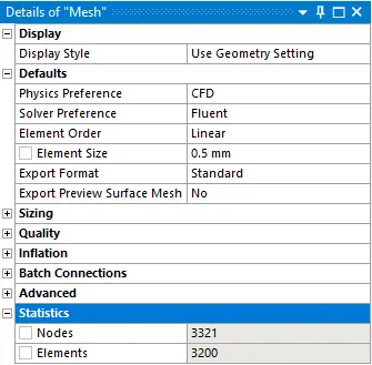
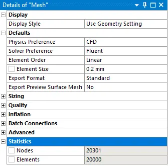
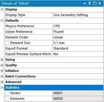
Following are the 3 Mesh Configurations for the Analysis.

Mesh Config. 1 -

Mesh Config. 2-

Mesh Config. 3-

Mesh Quality Verification-

Following is the surface mesh And Element quality of the Case Setup -

i) For Mesh Configuration 1 -

ii) For Mesh Configuration 2 -

iii) For Mesh Configuration 3 -

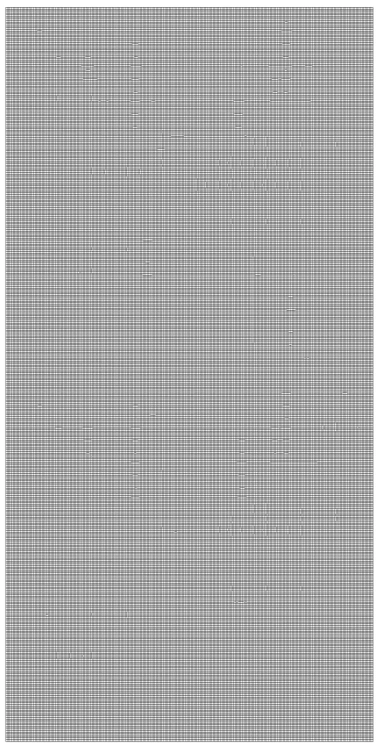
We can the mesh quality is very satisfied. 90% of the mesh cell are lying on good quality range.

3) Solver Settings -

Closing the Mesher & opening the Fluent Solver from the workbench

Checking the the Double precision option and selecting no. of parallel process.

Setting solver settings and initialization values.

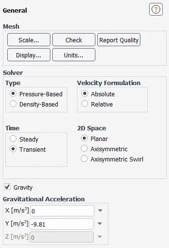
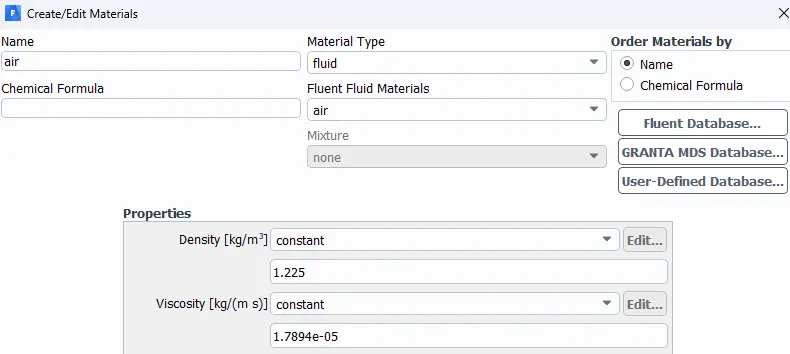
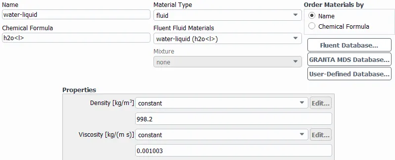
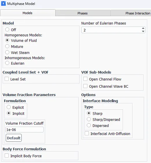
Selecting the VOF model and its settings.

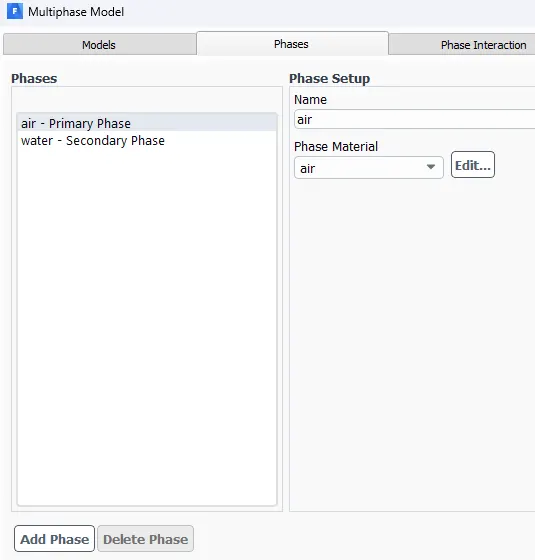
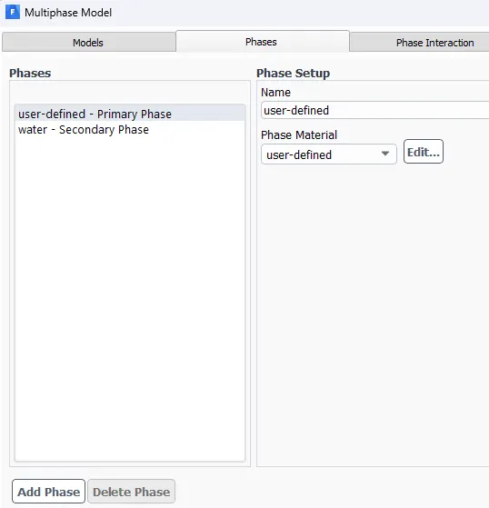
2nd case -

Setting Inilization, here we are using Hybrid Initialization.

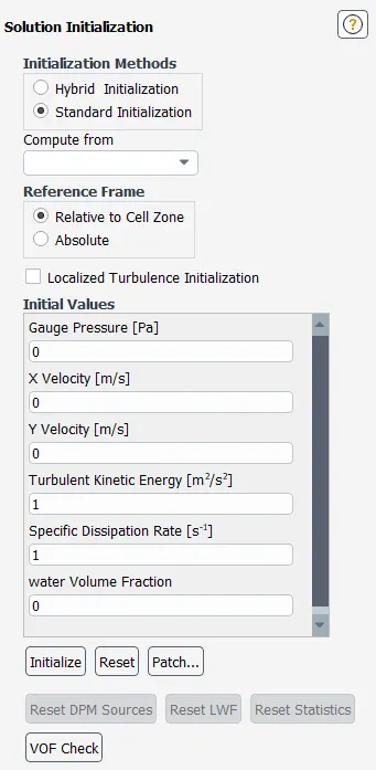
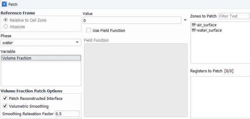
After Doing standard Initialize once we need to patch the phases of the regions via Volume fraction of a fluid i.e. Water here for both the cases.

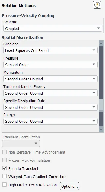
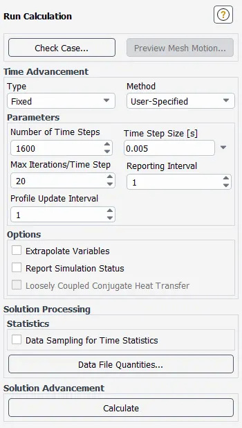
Keeping the Solution method & discretization schemes as shown below.

POST PROCESSING :

Outputs

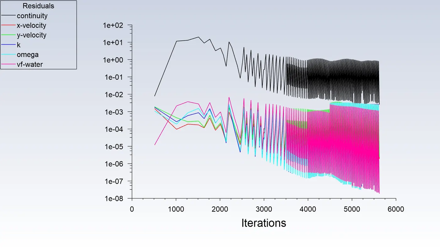
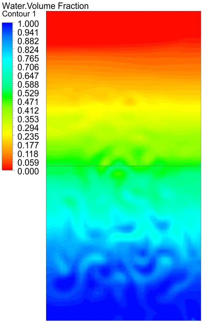
1. For Mesh Config. 1 (Water-Air)-

Residuals and Solution Plot -

Animation -

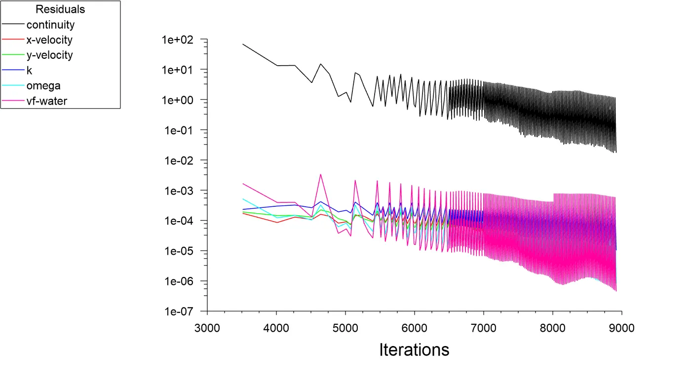
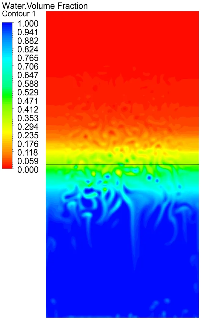
2. For Mesh Config. 2 (Water-Air)-

Residuals and Solution Plot -

Animation -

2. For Mesh Config. 3 (Water-Air)-

Residuals and Solution Plot -

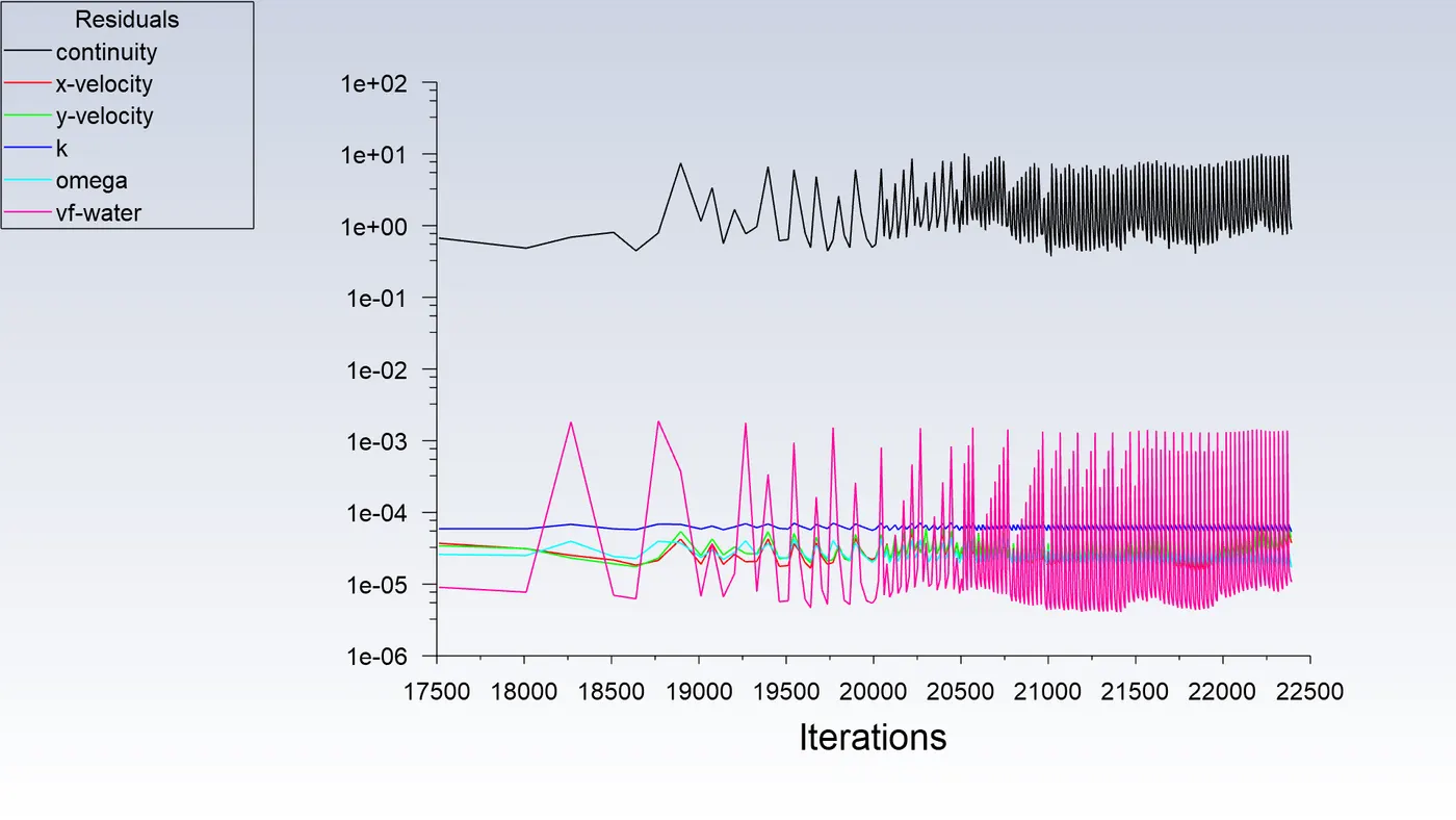
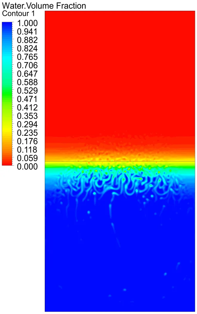
Animation -

4. For Mesh Config. 3 (Water-User Defined fluid of density = 400kg/m3) -

Residuals and Solution Plot -

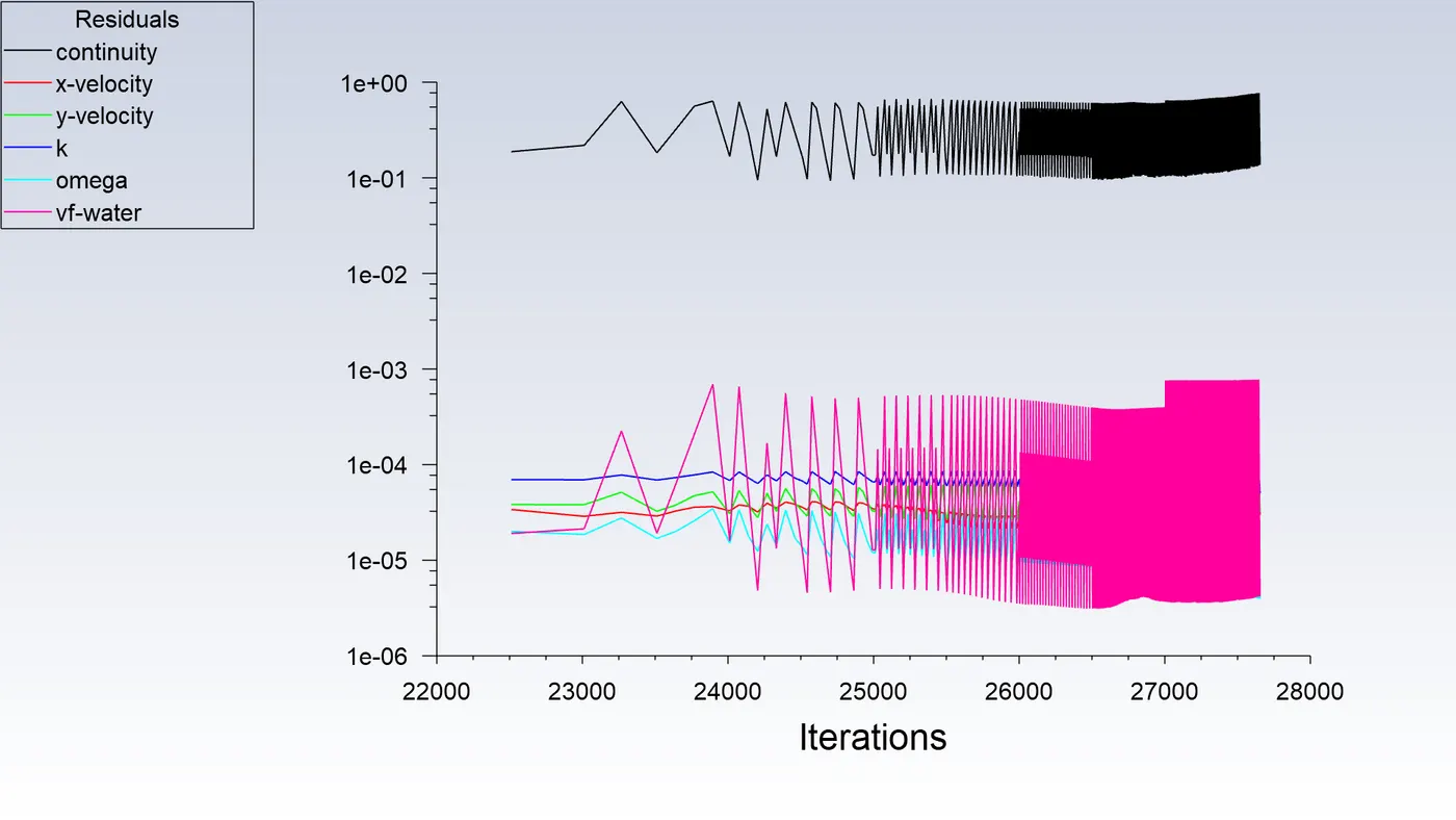
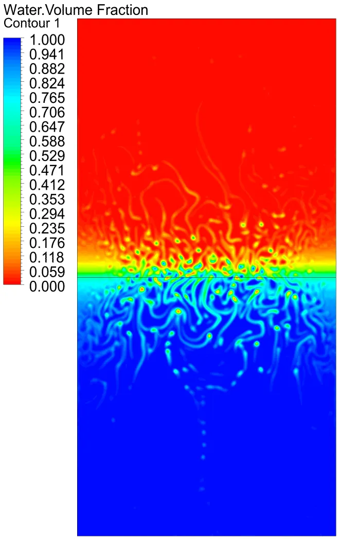
Animation -

RESULTS :

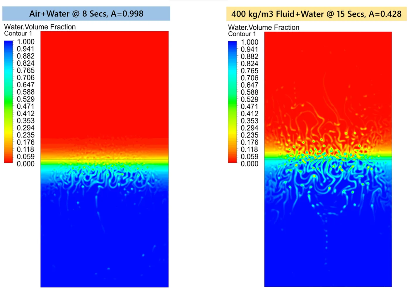
Following are the atwood no. for the 2 different cases which we are analysing -

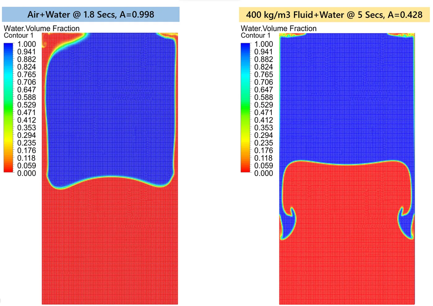
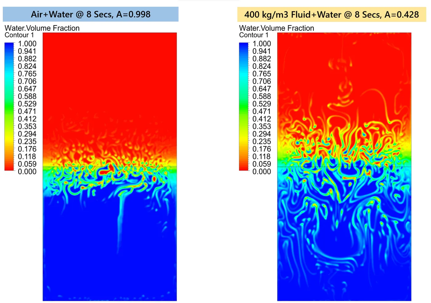
The Following are the state of the fluids for comparison of the above atwood no. cases and at different timesteps -

CONCLUSION :

We have successfully performed the Rayleigh Taylor stabilty analysis using Volume of Fluid Method in Ansys fluent.

The solver was set up using suitable settings to incorporate the physical phenomena.

We were able to generate required contours for for volume of fluid.

The following conclusions can be drawn based on the simulation results after running -

- we observe that finer mesh captures the instability better than the coarse mesh, and we run the the model for every time step of 0.005sec, due to this the computational time is long. VOF method results requires finer mesh for acurate results.

- From the results we can observe that, for the Atwood number close to 0, RT instability flows take the form of symmetric fingers of fluid, and also when Atwood number close to 1, the much lighter fluid below the heavier fluid takes the form of larger bubble-like plumes.

- Also we can observe that, for the atwood no. closer to 0, RT instabilty flow resolves/dissolves more slowly than for higher atwood no. , because when the viscosity of the fluid is high then the reynolds is very low and so less turbulence and therefore slow mixing of the fluid.

REFERENCE :

1. Rayleigh-Taylor Instability - https://www.youtube.com/watch?v=bW4526vHnY0
2. When Two Fluids Meet - A Rayleigh-Taylor Instability - https://youtu.be/EAJPtBSUoLw?si=h-zX9eCGkqOuvYbW
3. Malcolm J. Andrews and Stuart B. Dalziel;'Small Atwood number Rayleigh–Taylor experiments' - https://royalsocietypublishing.org/doi/10.1098/rsta.2010.0007
4. Suyeon Shin, Sung-Ik Sohn, Woonjae Hwang; 'Numerical simulation of single- and multi-mode Rayleigh–Taylor instability with surface tension in two dimensions'- https://doi.org/10.1016/j.euromechflu.2021.10.005