Partial Differential Equations : Its Types, Boundary and Initial Conditions
In ordinary differentiation, all the variables are differentiated with respect to the considered variable.
For example- Consider function, `f= ax^2 + by +z`
It's differentiation with respect to x is , `(df)/(dx) = 2ax + b(dy)/(dx) +(dz)/(dx)`
In partial differentiation, only the variable with respect to which the the function is being differentiated is considered as variable and other variables are considered as constants.
For example- Consider same function, `f= ax^2 + by +z`
It's partial derivate with respect to x is , `(delf)/(delx) = 2ax`
Ordinary differential equation (ODE) is a differential equation containing one or more functions of one independent variable and the derivatives of those functions.
For Example - Equation for motion of simple pendulum.
`(d^2theta)/(dt^2) + b/m(d theta)/(dt) +g/l sintheta = 0`
where `theta` = Angular Displacement
t = Time
b = Damping Coefficient
m = Mass of the Bob
g = Acceleration due to Gravity
l = length of the pendulum
we can see here, the Differential equation consist of derivatives of a dependent variable '`theta`' with only independent variable 't'.
Partial differential equation (PDE) is a differential equation containing partial derivatives of the dependent variable (one or more) with more than one independent variable.
For Example - The 1D Heat Equation
`(delT)/(delt) = k(del^2T)/(delx^2)`
where k = Thermal Diffusivity
T = Temperature (in K), Function of x and t, i.e. T(x,t)
t = time
we can see here, the Differential equation consitss of 2 partial derivatives of a dependent variable 'T' with the two independent variables 'x' and 't'.
Boundary conditions (B.C) are constraints necessary for the solution of a boundary value problem. A boundary value problem is a differential equation (or system of differential equations) to be solved in a domain on whose boundary a set of conditions is known.They arise naturally in every problem based on a differential equation to be solved in space.

Initial Conditions (I.C) are similiar to Boundary conditions but for the initial value problem. Initial value problems usually refer to problems to be solved in time. But on the other hand in many cases problem which is based on space and also with change with time, the problem is defined by the both initial conditions and boundary conditions.
Initial conditions and Boundary conditions can be understand by the Following Example
Taking the same above PDE for example of -
The 1D Heat Equation
`(delT)/(delt) = k(del^2T)/(delx^2)`
where k = Thermal Diffusivity
T = Temperature (in K), Function of x and t, i.e. T(x,t)
t = time
Consider a rod of length L with insulated sides is given an initial temperature distribution of f(x) degree C, for 0 < x < L . Find u(x,t) at subsequent times t>0 if end of rod are kept at 0 degree C.
The Heat Eqn and corresponding IC and BCs are thus,
PDE : `(delT)/(delt) = k(del^2T)/(delx^2)`, `0 < x < L`
I.C. : `T(x,0) =f(x)`, `0 < x < L`
B.C. : `T(0, t) =T(L, t) = 0`, `t > 0`
Why do we Need Boundary and Initial conditions?
Boundary value problems are extremely important as they model a vast amount of phenomena and applications, from solid mechanics to heat transfer, from fluid mechanics to acoustic diffusion. They arise naturally in every problem based on a differential equation to be solved in space, while initial value problems usually refer to problems to be solved in time.
Types of Boundary Conditions
Both ordinary and partial differential equations need boundary conditions to be solved. Different types of boundary conditions can be imposed on the boundary of the domain. The choice of the boundary condition is fundamental for the resolution of the computational problem: a bad imposition of b.c. may lead to the divergence of the solution or to the convergence to a wrong solution.
a) Dirichlet Boundary Condition
A boundary condition which specifies the value of the function itself is a Dirichlet boundary condition. This Condition Specifies the value that the unknown function needs to take on along the boundary of the domain. For example, if one end of an iron rod is held at absolute zero, then the value of the problem would be known at that point in space.
b) Neumann Boundary Condition
A boundary condition which specifies the value of the normal derivative of the function is a Neumann boundary condition. When imposed on an ordinary or a partial differential equation, the condition specifies the values of the derivative applied at the boundary of the domain. For example, if there is a heater at one end of an iron rod, then energy would be added at a constant rate but the actual temperature would not be known.
c) Robin Boundary Condition
When imposed on an ordinary or a partial differential equation, it is a specification of a linear combination of the values of a function and the values of its derivative on the boundary of the domain.
Robin boundary conditions are also called impedance boundary conditions, from their application in electromagnetic problems, or convective boundary conditions, from their application in heat transfer problems
d) Mixed Boundary Condition
A mixed boundary condition for a partial differential equation defines a boundary value problem in which the solution of the given equation is required to satisfy different boundary conditions on disjoint parts of the boundary of the domain where the condition is stated. It consists of applying different types of boundary conditions in different parts of domain.
Precisely, in a mixed boundary value problem, the solution is required to satisfy a Dirichlet or a Neumann boundary condition in a mutually exclusive way on the whole boundary of a given domain.
e) Cauchy Boundary Condition
Cauchy boundary condition augments an ordinary differential equation or a partial differential equation with conditions that the solution must satisfy on the boundary; ideally so to ensure that a unique solution exists. A Cauchy boundary condition specifies both the function value and normal derivative on the boundary of the domain. This corresponds to imposing both a Dirichlet and a Neumann boundary condition.
Different Classes of PDEs
The different types of partial differential equations are:
i) First-order Partial Differential Equation -
The order of a PDE is determined by the highest derivative in the equation. The First-order equation would be whose highest derviative be 1.
`(del phi)/(delx)+(del phi)/(dely) = 0`
ii) Linear Partial Differential Equation -
A linear PDE is one that is of first degree in all of its field variables and partial derivatives. For example,
`(del phi)/(delx)+(del phi)/(dely) = 0`
and so, the non-linear PDE can be-
`(del phi)/(delx)+((del phi)/(dely))^2 = 0`
iii) Quasi-Linear Partial Differential Equation -
A PDE is said to be quasi-linear if all the terms with the highest order derivatives of dependent variables occur linearly, that is the coefficient of those terms are functions of only lower-order derivatives of the dependent variables. However, terms with lower-order derivatives can occur in any manner. Eg-
`(del^2phi)/(delx^2)+phi(del^2phi)/(dely^2) = 0`
iv) Homogeneous Partial Differential Equation -
If all the terms of a PDE contain the dependent variable or its partial derivatives then such a PDE is called non-homogeneous partial differential equation or homogeneous otherwise.
in other words, A differential equation is homogeneous if it contains no non-differential terms and heterogeneous if it does.
Eg-
Homogeneous PDE -
`(del^2 phi)/(delx^2)+(del^2 phi)/(dely^2) = 0`
And
Non-Homogenous PDE can be -
`(del^2 phi)/(delx^2)+(del^2 phi)/(dely^2) + (del^2 phi)/(delxdely)= x^2+y^2`
Types on Behaviour of PDEs -
The solution depends on the equation and several variables contain partial derivatives with respect to the variables. There are three-types of second-order PDEs in mechanics. These are distinguished by two principal categories of physical behaviour:
• Equilibrium problems (Steady State problems, that do not changes with space and time)
- Elliptic Equation
• Marching problems ( The are transient problems, that do changes with space and time)
- Parabolic Equation
- Hyperbolic Equation
1) Elliptic PDE
Elliptic PDEs are mostly for steady state situations. For e.g. the steady state distribution of temperature in a rod of solid material or the equilibrium stress distribution of a solid object under a given applied load, as well as many steady fluid flows. These and many other steady state problems are governed by elliptic equations.
If the solution of the 2nd order PDE is, `b^2-ac < 0` then its a Elliptic solution.
The prototype elliptic equation can be given Laplace’s equation,
`(del^2phi)/(delx^2)+(del^2phi)/(dely^2) = 0`
A simple example of an equilibrium problem is the steady state heat conduction in equation in an insulated rod of metal by putting `phi = T`.
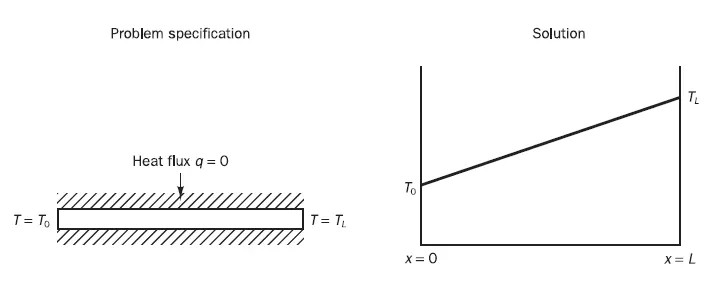
Steady State Heat Conduction in a Insulated Metal Rod
2) Parabolic PDE
Parabolic equations describe time-dependent problems, which involve significant amounts of diffusion. Examples are unsteady viscous flows and unsteady heat conduction.
If solution of the 2nd order PDE is, `b^2-ac = 0` then its a Parabolic solution.
The prototype parabolic equation can be given by the diffusion equation
`(del phi)/(del t) = k(del^2phi)/(delx^2)`
The transient distribution of temperature in an insulated rod of metal, can be represented by putting `phi = T` in the equation.
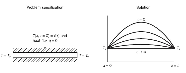
Transient distribution of temperature in an Insulated Metal Rod
3) Hyperbolic PDE
Hyperbolic equations dominate the analysis of vibration problems. In general they appear in time-dependent processes with negligible amounts of energy dissipation.
If solution of the 2nd order PDE is, `b^2-ac > 0` then its a Hyperbolic solution.
The prototype hyperbolic equation can be given by the wave equation.
`(del^2phi)/(delt^2) = c^2 (del^2phi)/(delx^2)`
The above form of the equation governs the transverse displacement (`phi = y`) of a string under tension during small-amplitude vibrations and also acoustic oscillations. The constant 'c' is the wave speed. It is relatively straightforward to compute the fundamental mode of vibration of a string of length 'L' using the equation.
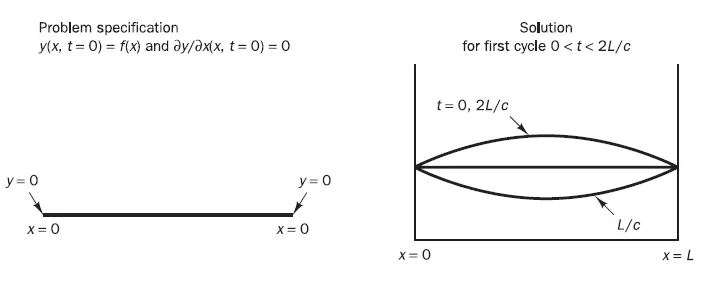
Vibrations of a string under tension