Finite Volume Method (FVM) - Literature Review (ITCFDUML&OF/Challenge/Week-9)
Computational fluid dynamics (CFD) is a branch of fluid mechanics that uses numerical analysis and data structures to analyze and solve problem that involves fluid flows. The fluid flow characteristics are very random and complex and usually defined by Navier-Stokes equations and Euler equations. These equations are in the differential and integral form, which are complex to feed into the computer as a part of input. Then there is need of discretizing those governing equation into an algebraic form, which can represent the governing equation in a numerical representation.
Discretization is the process through which we can transform continuous variables, models or functions into a discrete form. This process is usually carried out as a first step toward making them suitable for numerical evaluation.
There are different discretizing methods in Computational fluid dynamics. Some of the major discretization methods are:
1. Finite difference method
2. Finite volume method
3. Finite element method
Finite Difference Method (FDM) discretization is based upon the differential form of the PDE to be solved. Each derivative is replaced with an approximate difference formula (that can generally be derived from a Taylor series expansion). The computational domain is usually divided into hexahedral cells (the grid), and the solution will be obtained at each nodal point. The FDM is easiest to understand when the physical grid is Cartesian, but through the use of curvilinear transforms the method can be extended to domains that are not easily represented by brick-shaped elements. The discretization results in a system of equation of the variable at nodal points, and once a solution is found, then we have a discrete representation of the solution.
Finite-difference method is used in - Weather calculations, astrophysics, seismology, physical realism in computer graphics, and special effects.
Finite Volume Method (FVM) discretization is based upon an integral form of the PDE to be solved (e.g. conservation of mass, momentum, or energy). The PDE is written in a form which can be solved for a given finite volume (or cell). The computational domain is discretized into finite volumes and then for every volume the governing equations are solved. The resulting system of equations usually involves fluxes of the conserved variable, and thus the calculation of fluxes is very important in FVM. The basic advantage of this method over FDM is it does not require the use of structured grids, and the effort to convert the given mesh in to structured numerical grid internally is completely avoided. As with FDM, the resulting approximate solution is a discrete, but the variables are typically placed at cell centers rather than at nodal points. This is not always true, as there are also face-centered finite volume methods. In any case, the values of field variables at non-storage locations (e.g. vertices) are obtained using interpolation.
Finite-volume method mostly used in - CFD, heat transfer, and chemical engineering.
Finite Element Method (FEM) discretization is based upon a piecewise representation of the solution in terms of specified basis functions. The computational domain is divided up into smaller domains (finite elements) and the solution in each element is constructed from the basis functions. The actual equations that are solved are typically obtained by restating the conservation equation in weak form: the field variables are written in terms of the basis functions, the equation is multiplied by appropriate test functions, and then integrated over an element. Since the FEM solution is in terms of specific basis functions, a great deal more is known about the solution than for either FDM or FVM. This can be a double-edged sword, as the choice of basis functions is very important and boundary conditions may be more difficult to formulate. Again, a system of equations is obtained (usually for nodal values) that must be solved to obtain a solution.
Finite-element method is used in - All kinds of structural analysis, heat transfer, chemical engineering, electromagnetics (including electrostatics, magnetostatics, low-frequency electromagnetics, and frequency-domain high-frequency electromagnetic waves), multi-physics, and CFD.
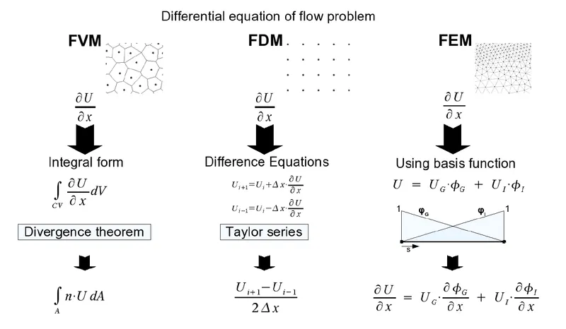
Why FVM for CFD?
The finite-volume method is a natural choice for CFD problems, since the partial differential equations you have to solve for CFD are conservation laws. However, both finite differences and finite elements can also be used for CFD. Efficient technology for CFD with the finite-element method has become increasingly popular over the last 10 to 15 years. Techniques for CFD with the finite-difference and finite-volume method have been known and used much longer.Finite volume methods can be compared and contrasted with the finite difference methods, which approximate derivatives using nodal values, or finite element methods, which create local approximations of a solution using local data, and construct a global approximation by stitching them together. In contrast a finite volume method evaluates exact expressions for the average value of the solution over some volume, and uses this data to construct approximations of the solution within cells.
The finite-volume method’s strength is that it only needs to do flux evaluation for the cell boundaries. This also holds for nonlinear problems, which makes it extra powerful for robust handling of (nonlinear) conservation laws appearing in transport problems.
The local accuracy of the finite-volume method, such as close to a corner of interest, can be increased by refining the mesh around that corner, similar to the finite-element method. However, the functions that approximate the solution when using the finite-volume method cannot be easily made of higher order. This is a disadvantage of the finite-volume method compared to the finite-element and finite-difference methods.
Seeing Differences between FDM and FVM from Steady-State 1D linear Heat Conduction Problem Example.
- 1D Heat Conduction by FDM -
In FDM basically,
- we divide domain in discrete cartesian points.
- The governing equation is solved at each point/node of the grid.
- Now for discretization, derivatives of the governing equation is replaced with an approximate difference formula that is generally derived from a Taylor series expansion.
General 1D heat conduction equation with source term(Heat Generation Term) ,
`alpha*(del^2T)/(delx^2) + S = 0`
where, T = Temperature, `alpha`= Thermal Diffusivity, and S =Source Term,
Source term here is Heat generation, given by S = g/k
'g'= Volumetric rate of internal heat generation, 'k' = Thermal Conductivity
Now for discretiztion we can consider the following diagram, showing the grid points of the domain.
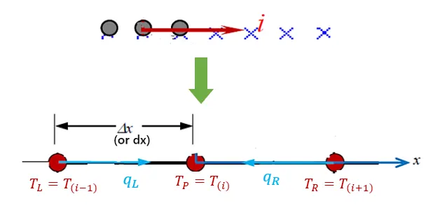
By applying 2nd order Central Differnce Approximation (Derived from taylor series Expansion),
we get the Discretized Equation to solve the problem numerically,
`alpha((T_(i+1) - 2(T_(i)) +T_(i-1) )/(dx^2)) + S = 0`
here for the simplicity, we have shown `alpha` and S Constant. However, Thermal Diffusivity is related to thermal conductivity and hence, is the function of temperature. Also source term here heat Generation, is also the function of temperature.
- 1D Heat Conduction using FVM
In Finite Volume method, instead of writing the equations in a point, we write it for the volume, and by applying few mathe techniques we are able to solve these equation for any type of grid.
The finite volume representation is meant to be more efficient in preserving the concept of conservation.
The Following figure shows the schematic diagram of the FVM Grid. Here the the domain is segmented into small cells i.e. control volume.
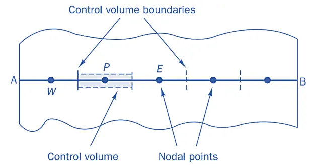
The values of the flux variables is stored at the centeroid of the control volume, which is the nodal point or node. This is basically known as cell-centered FVM method. In 2nd order FVM the values of these variables in the varies linearly control volume.
Following are the main key steps in FVM Discretization -
- Describing Governing equation in Integral Form - When we derive or write governing equation in PDE, that is usaully for a infinitesimally small fluid element, therefore for the control volume we need integrate the PDE governing equation of the fluid element to form governing equation for the control volume.
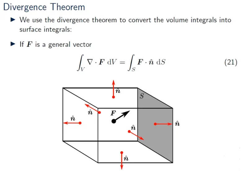
- Applying the Gauss-Divergence Theorem to the Integral form governing equation - the integral form we form for the governing equations is Volume Integral, Now we apply theGauss-Divergence Theorem that converts the volume integral to surface integral and vice versa, to account for the fluxes incoming and outgoing the control volume.
- Calculate Flux Terms by suitable methods - In a general the governing equation have convective terms, Diffusive terms, gradient terms and source terms (constant or varying). The integrals of these terms is solved individualy with suitable methods for them respectively. And finally we can to the Linear Algebriac Form which we solve computationaly.
Now for the 1-D Heat conduction problem, following diagram shows the schematics of cells grid distribution of domain -
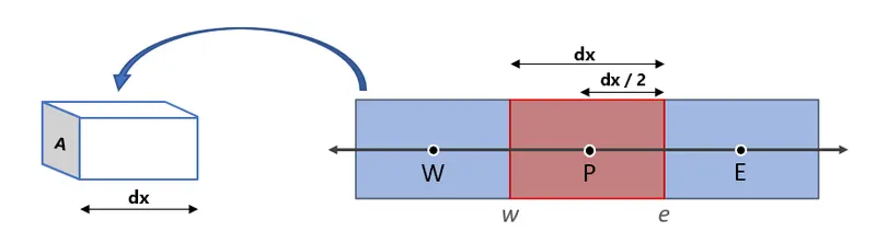
Here, the Heat is transfering from cell W to P to E. And currently we are studing the Cell 'P'.
The 1D heat conduction equation with source term(Heat Generation Term) is,
`alpha*(del^2T)/(delx^2) + S = 0` or `del/(delx)(alpha*(delT)/(delx)) + S = 0`
Now for the control volume / cell, the integral form is,
`int(del/(delx)(alpha*(delT)/(delx)) + S).dV = 0`
`int_w^e del/(delx)(alpha*(delT)/(delx)).dV + int_w^e S.dV = 0`
since dV = A.dx,
`int_w^e del/(delx)(alpha*(delT)/(delx)).A*dx + int_w^e S.dV = 0`
`implies` `[alpha*A*(delT)/(delx)]_w^e + [barS.dV]_w^e = 0`
Here `barS` is the average of the source term S from face 'w' to face 'e'. We are considering the value is varying linearly across the cell.
Further linearizing the `barS*dV` term as it is function of Temperature can be given as,
`barS*dV = S_u + S_pT_p`.
And also the thermal diffusivity(`alpha`) is function of temperature (which function of distance/position in conduction) can be given by using linear approximations,
`alpha_w = (alpha_W + alpha_P)/2` & `alpha_e = (alpha_P + alpha_E)/2`
Now, we are estimating values at the faces of w and e where the heat flux enters and exits respectively. Above the `alpha_w`& `alpha_e` are th values of thermal diffusivity at the in & out faces, estimated from the `alpha_W`,`alpha_P`& `alpha_E`which are thermal diffusivity at centroid of cells W, P, & E respectively.
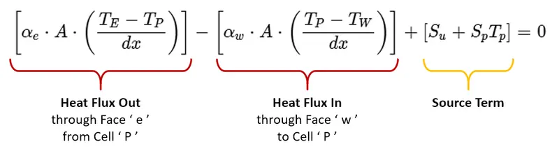
Hence the Discretized Equation of FVM for the problem is,
`alpha_e*A*((T_E-T_P)/dx) - alpha_w*A*((T_P-T_W)/dx) + S_u + S_pT_p = 0`
The fact about finite volume method is that the discretized equation has clear physical interpretation of the fluxes, convective, diffusive gradient and source terms. We can observe from the equation that the diffusive flux of T leaving the east face(e) minus the diffusive flux of T entering the west is equal to the generation of T i.e. it constitutes a balance equation for T over the control volume and clearly validates the conservation principle.
KEY CONCEPTS OF FVM - INTERPOLATION SCHEMES, GRADIENT SCHEMES, AND FLUX LIMITERS
A general Navier Stokes equation consists of Convection Terms, Diffusion Terms, Gradient Terms and Source terms.

The values of flux variables in general are calulated in the cell centroid. Now we need values of state variables at the faces of cell inorder to calculate flux passing through them. Also inorder calculate many other terms like source terms and gradiet terms we need value of some gradients.
INTERPOLATION SCHEMES
Many factors of the convective and diffusion terms are related to the value of flow(flux) variables such as T, p, U.
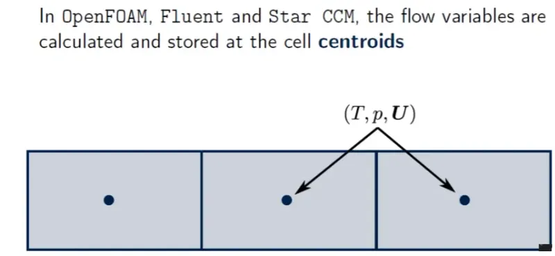
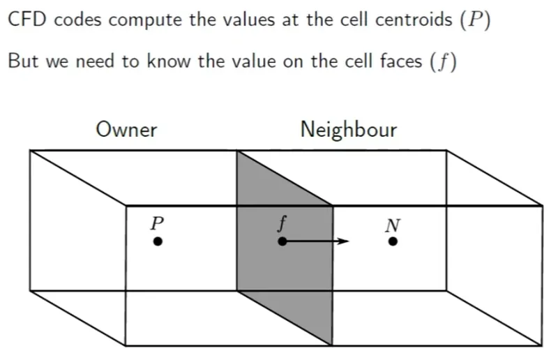
Now inorder to calculate the Fluxes and these terms at inlet & outlet faces we need to need to have the values of these state variables.
Therefore, we interpolate these state variables at the faces with reference to the values at the centroids. For example, Thermal conductivity and Thermal Diffusivtiy are function of Temperature, so we need to interpolate the Temperature at the face using value of cell centroid value.
The schemes or techniques used to interpolate and estimate the value at the face are known as Interpolation Schemes.
CFD code offer many different types of interpolation schemes,
- Upwind - first order accurate.
- Linear (Central differencing) - second order accurate, unbounded.
- Linear Upwind differncing(or Hybrid Differencing) - second order accurate, bounded.
- TVD - second order accurate, bounded.
- QUICK (Quadratic Upstream Interpolation for Convective Kinematics) - second order accurate
- limitedLinear - second order accurate, unbounded, but more stable than pure linear. (Recommended for LES simulations).
The CFD user must know which scheme to be used to solve and to simulate a given problem. As every scheme has different behaviour and application characteristics.
- First order methods are bounded and stable but diffusive.
- Second order methods are accurate, but they might become oscillatory.
- At the end of the day, most of the time want a second order accurate solution.
Understanding some common Interpolation schemes
For Understanding the schemes, let us consider the following setup,
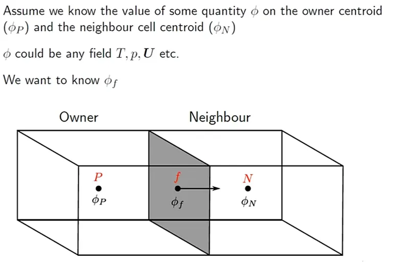
1. Upwind Scheme
This is the simplest numerical scheme. We assume that the value of f at the face is the same as the cell centered value in the cell upstream of the face. It depends on the direction mass flux.
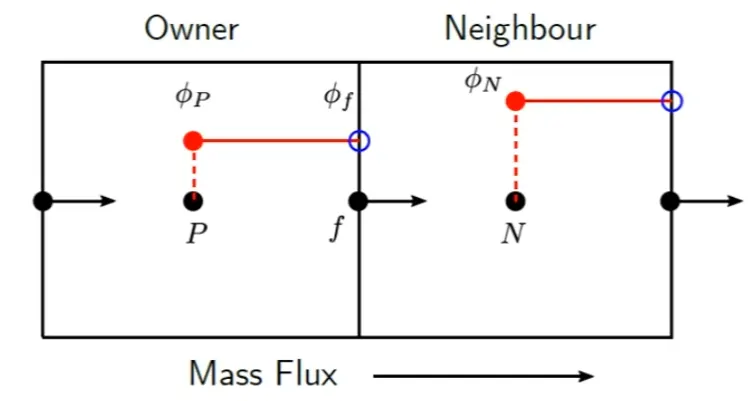
The main advantages are that it is easy to implement and that it results in very stable calculations, but it also very diffusive. Gradients in the flow field tend to be smeared out. This is often the best scheme to start calculations with.
2. Linear / Central differencing Scheme
This is an second order differencing scheme. It is basically the Linear interpolation. Most of the time in FVM we assume the value flow variables varying linearly across the cell. We know the value of the flow variables at the centeroids and the length between the centroids and faces, and therefore determine the value of the flow variables at the face by linear interpolation approximation.
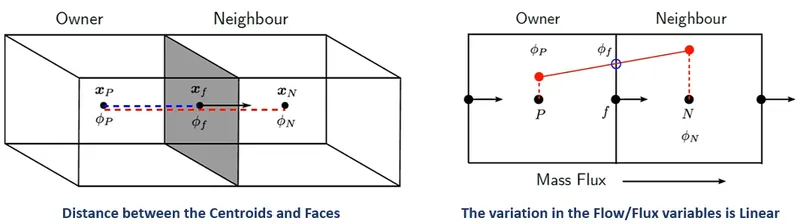
This is more accurate than the first order upwind scheme, but it leads to oscillations in the solution or divergence and thats why is often said to be ubounded.
These are often used to solve diffusion terms in the governing equation. Due to unbound characteristics it s avoid in the RANS solver for solving the convection terms.
3. Linear upwind Scheme
This is a very populer scheme for solving the convection terms. It is the hybrid of the Upwind scheme and the Linear scheme. But here we do not take the flux variable value at the face same as the centroid value like upwind and nor we interpolate like the central differencing.
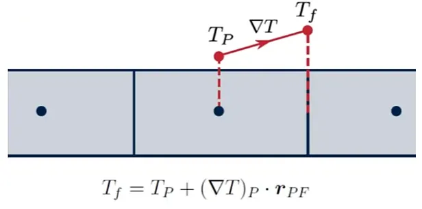
In linear-Upwind scheme we take the flux variable value of the cell centroid and extrapolate it to give value at the exit face. Inorder to improve the accuracy of the extrapolation we use the Gradient of the flow variable, which is Linear itself.
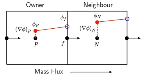
This scheme is more accurate than the upwind scheme and nominaly second-order accurate.
But this scheme can be unstable sometime, the reason can explanaed from the following case,
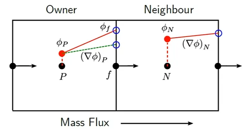
we can see here that due wrong or slight error in the extrapolation due inaccuracy in the gradient value can lead to the flux variable value at the face greater than the flux variable value of the upcoming centroid which is physically wrong and this can lead to the unstablity or divergence. Hence it is often recommend to run the simulation first with the first-order Upwind scheme and then Linear upwind.
Linear Upwind scheme is only meant to solve the Convection Terms, and avoided for the Diffusive terms in the governing equation.
And therefore inorder avoid the unstable results we require Gradient Schemes and Gradient Limiters.
More depth explanation - https://www.youtube.com/watch?v=JVE0fNkc540&ab_channel=FluidMechanics101
GRADIENT SCHEMES
In a typical governing equation there's need of gradient values of the flux variables for estimating terms and techniques.
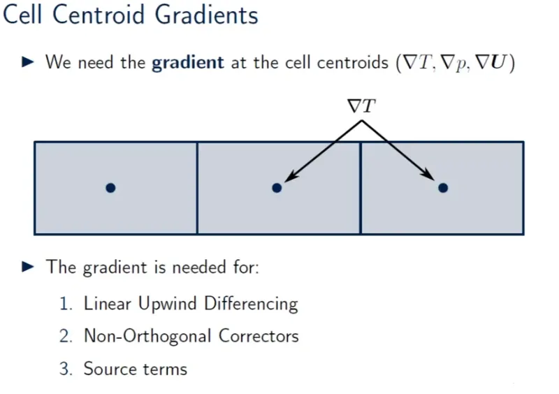
From the below short example case of conduction, the need of gradient in the linear upwind differencing,
In FVM, there are 3 most used gradient schemes -
- Green-Gauss Cell Based Method
https://www.youtube.com/watch?v=oeA1Bg9GqQQ&ab_channel=FluidMechanics101
- Green-Gauss Node Based Method
https://www.youtube.com/watch?v=tF_vrB3YLls&ab_channel=FluidMechanics101
- Least Square Method
https://www.youtube.com/watch?v=7ymFkxx2R_k&ab_channel=FluidMechanics101
FLUX LIMITERS
The Flux or Gradient limiter limits the sudden jump of rate of change of any flow quantity at cell face such that it is set between the values of both the cell centroids. Flux limiters are used in high resolution schemes – numerical schemes used to solve problems in science and engineering, particularly fluid dynamics, described by partial differential equations (PDE's). They are used in high resolution schemes, such as the MUSCL scheme, to avoid the spurious oscillations (wiggles) that would otherwise occur with high order spatial discretization schemes due to shocks, discontinuities or sharp changes in the solution domain. Use of flux limiters, together with an appropriate high resolution scheme, make the solutions total variation diminishing (TVD) .Flux limiters are also referred to as slope limiters because they both have the same mathematical form, and both have the effect of limiting the solution gradient near shocks or discontinuities. In general, the term flux limiter is used when the limiter acts on system fluxes and slope limiter is used when the limiter acts on system states (like pressure, velocity etc.).
The main idea behind the construction of flux limiter schemes is to limit the spatial derivatives to realistic values for scientific and engineering problems this usually means physically realisable and meaningful values. They are used in high resolution schemes for solving problems described by PDEs and only come into operation when sharp wave fronts are present. For smoothly changing waves, the flux limiters do not operate and the spatial derivatives can be represented by higher order approximations without introducing spurious oscillations.
REFERENCE :
https://www.cfd-online.com/Forums/fluent/39028-difference-between-fem-fdm-fvm.html
https://www.youtube.com/watch?v=Kl-CpfA2gSU
https://www.youtube.com/watch?v=E9_kyXjtRHc&ab_channel=FluidMechanics101
https://www.youtube.com/watch?v=JVE0fNkc540&ab_channel=FluidMechanics101
Fluid Mechanics 101 - https://www.youtube.com/channel/UCcqQi9LT0ETkRoUu8eYaEkg/videos