MATLAB Program to fit a polynomial for the given Cp vs Temperature Experimental Data & Measure the Accuracy of the Curve Fit. (Matlab/Challenge-Week 4-Curve Fitting)
AIM: Write a code to fit a linear and cubic polynomial for the given Cp vs Temperature Data.
OBJECTIVE:
- A MATLAB Code to fit a polynomial for the given data.
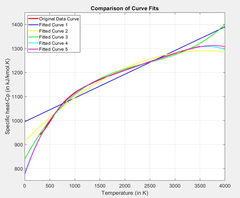
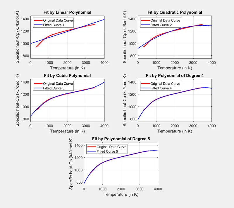
- Plot the comparison curves for the fitted polynomials with respect to the curve of original data.
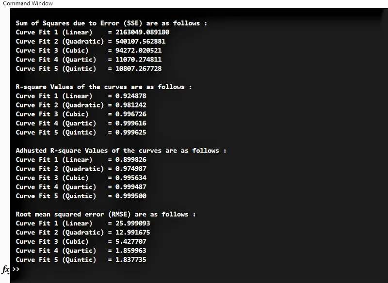
- Measure the accuracy of the fitted curve with respect to the original data curve.
THEORY:
There are different ways to represent data generated by a system. Data generated by a system due to variation in the variables it can be presented in a graphical form, more specifically the forming curves by the plotted data point. By this, it becomes easier to observe or understand the characteristics of a system.
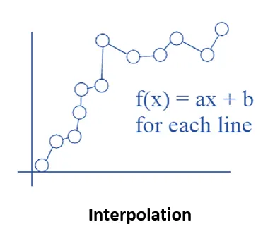
Interpolation - is a type of estimation, a method of constructing new data points within the range of a discrete set of known data points. In engineering and science, one often has a number of data points, obtained by sampling or experimentation, which represent the values of a function for a limited number of values of the independent variable. It is often required to interpolate, i.e., estimate the value of that function for an intermediate value of the independent variable.
If data is reliable, it can be plotted by connecting the dots. This is piece-wise, linear interpolation. This has limited use as a general function f(x). Since its really a group Of small f (x)s, connecting one point to the next it doesn't work very well for data that has a built-in random error (scatter). A general representation of the interpolation can be seen as,
Curve Fitting -
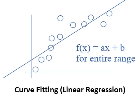
Curve fitting is the process of constructing a curve, or mathematical function, that has the best fit to a series of data points, possibly subject to constraints. It is the way we model or represent a data spread by assigning the best fit function (curve) along the entire range. Ideally, it will capture the trend in the data by assigning a single function across the entire range and allow us to make predictions of how the data series will behave in the future.
A general graphical curve fitting for a simple linear equation f(x)= ax + b can be seen as below,
A related topic is regression analysis, which focuses more on questions of statistical inference such as how much uncertainty is present in a curve that is fit to data observed with random errors. Fitted curves can be used as an aid for data visualization, to infer values of a function where no data are available, and to summarize the relationships among two or more variables.
Regression is a method of estimating the relationship between a response (output) variable and one or more predictor (input) variables. You can use linear and nonlinear regression to predict, forecast, and estimate values between observed data points.
Linear curve fitting, or linear regression, is when the data is fit to a straight line ( function of - f(x)= a x + b). Although there might be some curve to your data, a straight line provides a reasonable enough fit to make predictions.

Linear regression models are often fitted using the least squares approach, the least squares method is a statistical procedure to find the best fit for a set of data points by minimizing the sum of the offsets or residuals of points from the plotted curve.
Considering the vertical distance from each point to a prospective line as an error, and summing them up over our range, gives us a concrete number that expresses how far from ‘best’ the prospective line is.
Since it’s the offset or distance from our points to the line we’re interested in, whether it is positive or negative distance is not relevant, we square the distance in our error calculations. This also allows us to weight greater errors more heavily. So this method is called the least squares approach.
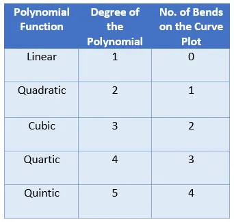
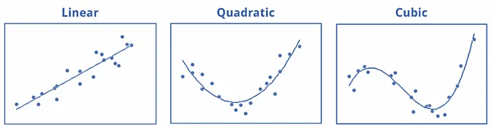
Polynomial curve fitting is when we fit our data to the graph of a polynomial function. The same least squares method can be used to find the polynomial, of a given degree, that has a minimum total error. polynomial regression is a form of regression analysis in which the relationship between the independent variable x and the dependent variable y is modelled as an nth degree polynomial in x.
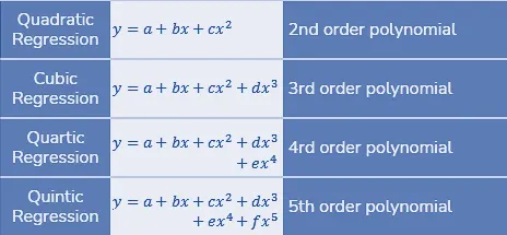
One of the characteristics of algebra or polynomials is that, as we increase the degree of polynomial, the no. of bends on the curves increases.
Estimation of Goodness of the Fit :
Apart from the graphical methods to evaluate the goodness of fit, the goodness of fit statistics can be examined out for
optimising the curve fit. The Curve Fitting Toolbox supports different measures Of goodness Of fit statistics for parametric
models, they are:
- Sum of squares due to error (SSE)
- R-square (`R^2`)
- Adjusted R-square (`R_(Adj)^2`)
- Root mean squared error (RMSE)
1. Sum of squares due to error (SSE)
This statistic measures the total deviation of the response values from the fit to the response values. It is also called the
summed square of residuals and is usually labelled as SSE.
Error = `| y_i-`value of `f(x)` at `x_i`| = `|y_i-f(x_i)|`
where, i = `1` to `n^(th)`
`y_i` is the original datapoint with respect to x-axis variable
`f(x_i)` is the datapoint of function of curve fit with respect to x-axis variable
SSE = `sum_(i=1)^n``|y_i-f(x_i)|^2`
SSE value closer to 0 indicates a better fit.
2. R-square (`R^2`)
This statistic measures how successful the fit is in explaining the variation of the data. Put another way, R-square is the square of the correlation between the response values and the predicted response values. It is also called the square of the multiple correlation coefficient and the coefficient of multiple determination. R-square is defined as the ratio of the sum of squares of the regression (SSR) and the total sum of squares (SST).
if `y = f(x)` is the fit curve then the SSR is defined as follows,
SSR = `sum_(i=1)^n``|f(x_i)-bary|^2`, where `bary` is the mean of the response value y.
Now the term SST is given by the summation of SSR and SSE,
SST = SSR + SSE
From here, we can calculate the value of `R^2`,
`R^2 = (SSR)/(SST)` or `R^2 = 1-(SSE)/(SST)`
`R^2` value closer to 1 indicates a better curve fit.
3. Adjusted R-square (`R_(Adj)^2`)
Adjusted R-square disregards these infinitesimally small increments to R-square, and only considers the variables which actually contribute to the output of the system in a drastic way. R-square is formulated as shown below,
`R_(Adj)^2 = 1-[(SSE(n-1))/(SST(k-1))]`
or
`R_(Adj)^2 = 1-[((1-R^2)(n-1))/(n-k-1)]`
where,
n - the number of data points
k - the number of independent variables
`R_(Adj)^2` value closer to 1 indicates a better curve fit.
4. Root mean squared error (RMSE)
This statistic is also known as the fit standard error and the standard error of the regression. It is an estimate of the standard deviation of the random component in the data, and is defined as,
`RMSE = root .((sum_(i=0)^n(y_i-f(x_i))^2)/n) = root.((SSE)/n)`
where,
n - is the total number of data points available.
RMSE value closer to 0 indicates a better curve fit.
PROGRAM :
- Following is the program's Main function -
% ------------------------------- Matlab Program for estimating the curve fit ----------------------------- clear all close all clc % Loading Data from the File cp_data = load('data'); temp = cp_data(:,1); cp = cp_data(:,2); T = [1:4000]; % Temp. Variable (X-axis Variable) Range for the Fitted Cp % forming for Linear polynomial [coeffs1,s,mu] = polyfit(temp,cp,1); % forming polynomial(taking coefficients) using experiment data fitted_cp1 = polyval(coeffs1, T, s, mu); % predicting cp from temp. by the formed polynomial [sse1, rsq1, arsq1, rmse1] = fit_error_calc(cp,temp,fitted_cp1,T); % calling fitness error calculation function inorder obtain the goodness of the fit % for Quadratic polynomial [coeffs2,s,mu] = polyfit(temp,cp,2); fitted_cp2 = polyval(coeffs2, T, s, mu); [sse2, rsq2, arsq2, rmse2] = fit_error_calc(cp,temp,fitted_cp2,T); % for Cubic polynomial [coeffs3,s,mu] = polyfit(temp,cp,3); fitted_cp3 = polyval(coeffs3, T, s, mu); [sse3, rsq3, arsq3, rmse3] = fit_error_calc(cp,temp,fitted_cp3,T); % for polynomial with degree of 4 [coeffs4,s,mu] = polyfit(temp,cp,4); fitted_cp4 = polyval(coeffs4, T, s, mu); [sse4, rsq4, arsq4, rmse4] = fit_error_calc(cp,temp,fitted_cp4,T); % for polynomial with degree of 5 [coeffs5,s,mu] = polyfit(temp,cp,5); fitted_cp5 = polyval(coeffs5, T, s, mu); [sse5, rsq5, arsq5, rmse5] = fit_error_calc(cp,temp,fitted_cp5,T); % -------------------- Goodness of the fit ---------------------- fprintf('n Sum of Squares due to Error (SSE) are as follows : n'); fprintf(' Curve Fit 1 (Linear) = %f n',sse1); fprintf(' Curve Fit 2 (Quadratic) = %f n',sse2); fprintf(' Curve Fit 3 (Cubic) = %f n',sse3); fprintf(' Curve Fit 4 (Quartic) = %f n',sse4); fprintf(' Curve Fit 5 (Quintic) = %f n',sse5); fprintf('n R-square Values of the curves are as follows : n'); fprintf(' Curve Fit 1 (Linear) = %f n',rsq1); fprintf(' Curve Fit 2 (Quadratic) = %f n',rsq2); fprintf(' Curve Fit 3 (Cubic) = %f n',rsq3); fprintf(' Curve Fit 4 (Quartic) = %f n',rsq4); fprintf(' Curve Fit 5 (Quintic) = %f n',rsq5); fprintf('n Adhusted R-square Values of the curves are as follows : n'); fprintf(' Curve Fit 1 (Linear) = %f n',arsq1); fprintf(' Curve Fit 2 (Quadratic) = %f n',arsq2); fprintf(' Curve Fit 3 (Cubic) = %f n',arsq3); fprintf(' Curve Fit 4 (Quartic) = %f n',arsq4); fprintf(' Curve Fit 5 (Quintic) = %f n',arsq5); fprintf('n Root mean squared error (RMSE) are as follows : n'); fprintf(' Curve Fit 1 (Linear) = %f n',rmse1); fprintf(' Curve Fit 2 (Quadratic) = %f n',rmse2); fprintf(' Curve Fit 3 (Cubic) = %f n',rmse3); fprintf(' Curve Fit 4 (Quartic) = %f n',rmse4); fprintf(' Curve Fit 5 (Quintic) = %f n',rmse5); %.................. Graphical Comparion..................... figure(1) plot(temp,cp,'linewidth',3,'color','r'); hold on; grid on; plot(T,fitted_cp1,'linewidth',2,'color','b'); plot(T,fitted_cp2,'linewidth',2,'color','y'); plot(T,fitted_cp3,'linewidth',2,'color','g'); plot(T,fitted_cp4,'linewidth',2,'color','c'); plot(T,fitted_cp5,'linewidth',2,'color','m'); axis([0 4000 750 1450]); title('Comparison of Curve Fits'); xlabel('Temperature (in K)'); ylabel('Specific heat-Cp (in kJ/kmol.K)'); legend('Original Data Curve','Fitted Curve 1','Fitted Curve 2','Fitted Curve 3','Fitted Curve 4','Fitted Curve 5','location','northwest'); figure(2) subplot(11,7,[1,2,3,8,9,10,15,16,17]); plot(temp,cp,'linewidth',3,'color','r'); hold on; grid on; plot(T,fitted_cp1,'linewidth',2,'color','b'); axis([0 4000 750 1450]); title('Fit by Linear Polynomial'); xlabel('Temperature (in K)'); ylabel('Specific heat-Cp (kJ/kmol.K)'); legend('Original Data Curve','Fitted Curve 1','location','northwest'); subplot(11,7,[5,6,7,12,13,14,19,20,21]); plot(temp,cp,'linewidth',3,'color','r'); hold on; grid on; plot(T,fitted_cp2,'linewidth',2,'color','b'); axis([0 4000 750 1450]); title('Fit by Quadratic Polynomial'); xlabel('Temperature (in K)'); ylabel('Specific heat-Cp (kJ/kmol.K)'); legend('Original Data Curve','Fitted Curve 2','location','northwest'); subplot(11,7,[29,30,31,36,37,38,43,44,45]); plot(temp,cp,'linewidth',3,'color','r'); hold on; grid on; plot(T,fitted_cp3,'linewidth',2,'color','b'); axis([0 4000 750 1450]); title('Fit by Cubic Polynomial'); xlabel('Temperature (in K)'); ylabel('Specific heat-Cp (kJ/kmol.K)'); legend('Original Data Curve','Fitted Curve 3','location','northwest'); subplot(11,7,[33,34,35,40,41,42,47,48,49]); plot(temp,cp,'linewidth',3,'color','r'); hold on; grid on; plot(T,fitted_cp4,'linewidth',2,'color','b'); axis([0 4000 750 1450]); title('Fit by Polynomial of Degree 4'); xlabel('Temperature (in K)'); ylabel('Specific heat-Cp (kJ/kmol.K)'); legend('Original Data Curve','Fitted Curve 4','location','northwest'); subplot(11,7,[59,60,61,66,67,68,73,74,75]); plot(temp,cp,'linewidth',3,'color','r'); hold on; grid on; plot(T,fitted_cp5,'linewidth',2,'color','b'); axis([0 4000 750 1450]); title('Fit by Polynomial of Degree 5'); xlabel('Temperature (in K)'); ylabel('Specific heat-Cp (kJ/kmol.K)'); legend('Original Data Curve','Fitted Curve 5','location','northwest'); - Following is a function which Estimates Parameters Defies the Goodness of the Curve Fit -
% ------------- Function to Calculate goodness of the curve fit----------- function [sse, rsq, arsq, rmse] = fit_error_calc(cp,temp,f_cp,T) cp_sum = 0; sse = 0; ssr = 0; n = length(cp); % n - the number of data points k = length(f_cp) - length(cp); % k - the number of independent variables for i = 1 : length(cp) cp_sum = cp_sum + cp(i); end cp_mean = cp_sum/length(cp); % mean of all values of original Cp data for i = 1 : length(temp) if temp(i) == T(i+299) error = cp(i) - f_cp(i+299); sse = sse + (error^2); % sse is Sum of Squares due to Error (SSE) ssr = ssr + (f_cp(i+299) - cp_mean)^2; % ssr is squares of the regression (SSR) end end sst = sse + ssr; % sst is total sum of squares (SST) rsq = ssr/sst; % rsq is R-square Values of the curve arsq = 1 - ( ((1-rsq)*(n -1)) / (n-k-1) ); % arsq is Adhusted R-square Values of the curve rmse = (sse/n)^(1/2); % rmse is Root mean squared error (RMSE) end
OUTPUT :
Verifying the Curve Fit with the Curve Fitting Toolbox -
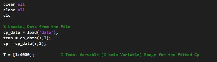
For using the Curve Fitting Toolbox First, we have to load the data from the file into the workspace by a piece of code as shown below -
Now, the toolbox can be used and perform curve fit as shown below -
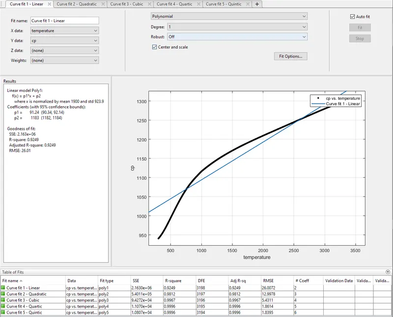
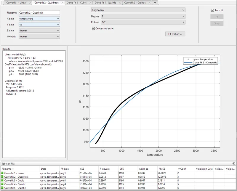
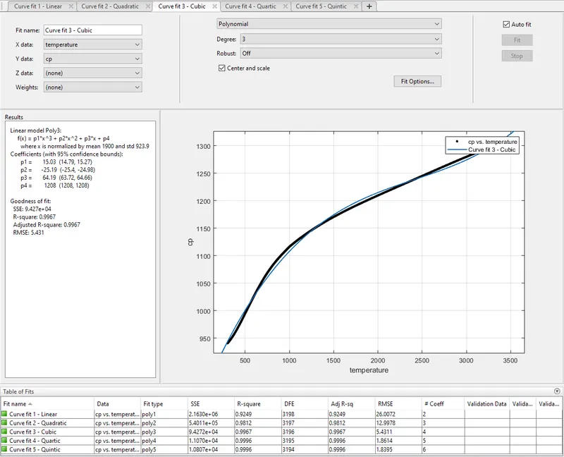
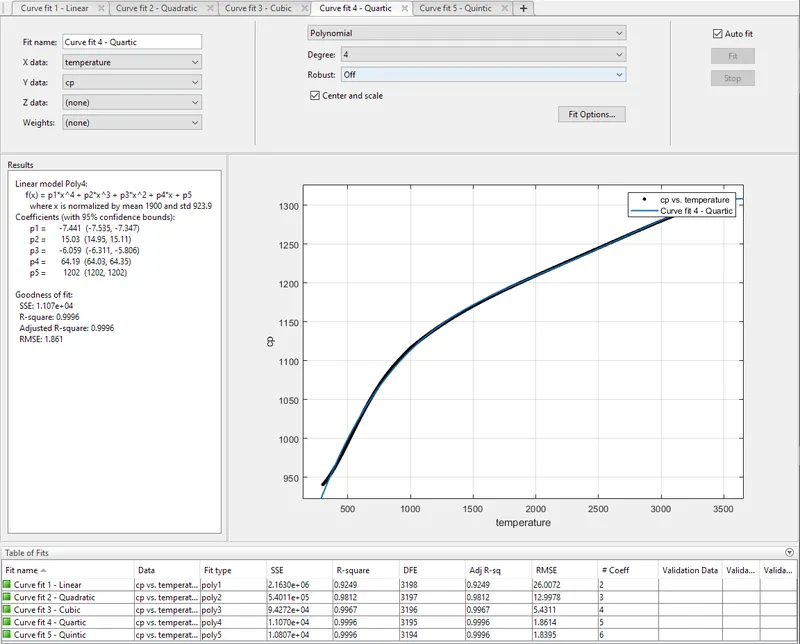
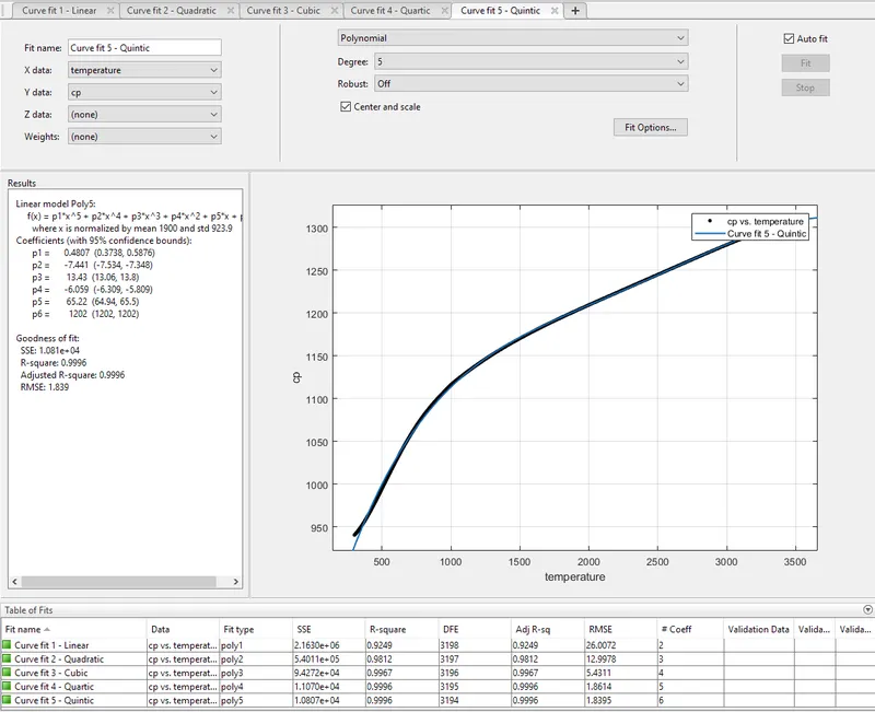
Hence, the Curve Fit goodness Parameter values i.e. SSE, R-square, Adj. R-square, and RMSE values of both the program and the Curve Fitting Toolbox matches with each other.
1) How to make a curve fit perfectly?
A perfect fit means, the curve should fit the original curve without showing any errors (such as centering and scaling errors) in that particular degree of the polynomial. That means it passes through every data points of the original data set and have 0 deviations. A perfect fit can always be the best fit but best fit can not be a perfect fit. To improve curve fit we use two methods first we increase degree of polynomial and second, we can use split wise method.
In order to get perfect fit, it should be well balanced between the degree of polynomial and no. of splits in data set. It usually non-efficient to obtain perfect fit, again it depends on the original data and the characteristics of that system obtaining data. If data is less complex, one may get perfect fit in 2-3 splits with quadratic or cubic polynomial. But, in case of complex, scattered and large no. of data points it becomes time inefficient.
That's why most of the time Best fit is obtained or considered.
2) How to get the best fit?
The best fit is the curve that best fits a set of coordinate plane points. It's the closest curves to the original data with very low errors/deviations from original data points. AS we know, to improve curve fit we use two methods first we increase the degree of polynomial and second, we use split wise method. So by obtain curve fit from this, we can get best fit by making use of Root mean squared error (RMSE) method to check the accuracy of the fit and then optimize it to get the least error i.e. best fit.
3) What could be done to improve the cubic fit?
In order to get best fit with cubic polynomial is to for Splitwise method.
Following is shown the fitting of the given problem by using cubic polynomial and splitwise method.
% --------- Matlab Program for estimating the curve fit using Splitwise Method and cubic Polynomial----------


clear all
close all
clc

% Loading Data from the File
cp_data = load('data');
temp = cp_data(:,1);
cp = cp_data(:,2);

% Splitting the Data, Assigning Loaded Data to a Specific Ranges
t1 = cp_data(1:500,1);
cp1 = cp_data(1:500,2);

t2 = cp_data(501:1000,1);
cp2 = cp_data(501:1000,2);

t3= cp_data(1001:2200,1);
cp3 = cp_data(1001:2200,2);

t4= cp_data(2201:3200,1);
cp4 = cp_data(2201:3200,2);

% Temp. Variable (X-axis Variable) Range for the Fitted Cp
T1 = [1:500];
T2 = [501:1000];
T3 = [1001:2200];
T4 = [2201:4000];

% Curve Fitting

[coeffs1,s,mu] =  polyfit(t1,cp1,3);      % forming polynomial(taking coefficients) using experiment data
fitted_cp1 = polyval(coeffs1, T1, s, mu); % predicting cp from temp. by the formed polynomial

[coeffs2,s,mu] =  polyfit(t2,cp2,3);
fitted_cp2 = polyval(coeffs2, T2, s, mu);

[coeffs3,s,mu] =  polyfit(t3,cp3,3);
fitted_cp3 = polyval(coeffs3, T3, s, mu);

[coeffs4,s,mu] =  polyfit(t4,cp4,3);
fitted_cp4 = polyval(coeffs4, T4, s, mu);

%.................. Graphical Comparion.....................
plot(temp,cp,'linewidth',3.5,'color','r');
hold on;    grid on;
plot(T1,fitted_cp1,'linewidth',2,'color','b');
plot(T2,fitted_cp2,'linewidth',2,'color','b');
plot(T3,fitted_cp3,'linewidth',2,'color','b');
plot(T4,fitted_cp4,'linewidth',2,'color','b');
axis([0 4000 750 1450]);
title('Curve Fitting by Splitwise Method using Cubic Polynomial');
xlabel('Temperature (in K)');
ylabel('Specific heat-Cp (kJ/kmol.K)');
legend('Original Data Curve','Fitted Curve','location','northwest');
Output -
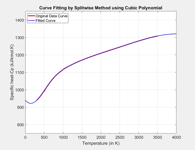
By Using Curve fitting Toolbox we got the Goodness Characteristics for the splitwise fit,

REFERENCES -
https://skill-lync.com/projects/Curve-Fitting-and-criterion-to-choose-best-fit-41860
https://www.statisticshowto.com/curve-fitting/
https://en.wikipedia.org/wiki/Curve_fitting
https://en.wikipedia.org/wiki/Regression_analysis
https://statisticsbyjim.com/regression/curve-fitting-linear-nonlinear-regression/
https://machinelearningmastery.com/curve-fitting-with-python/