Project 2 - Rankine cycle Simulator
AIM : To Create a Rankine Cycle Simulator using MATLAB.
OBJECTIVE :
- Code should calculate the state points of the Rankine Cycle (any type of your choice) based on user inputs.
- Plot the corresponding T-s and h-s plots for the given set of inputs.
- Should Calculate Net-work output, Back work ratio and Efficiency of the Rankine cycle.
THEORY :
Rankine cycle is an idealized thermodynamic cycle describing the process by which certain heat engines, such as steam turbines or reciprocating steam engines, allow mechanical work to be extracted from a fluid as it moves between a heat source and heat sink. The Rankine Cycle is named after William John Macquorn Rankine.
The Rankine cycle is the fundamental operating cycle of all power plants where an operating fluid is continuously evaporated and condensed. The selection of operating fluid depends mainly on the available temperature range.
Heat energy is supplied to the system via a Boiler where the working fluid (typically water) is converted to a high-pressure gaseous state (steam) in order to turn a Turbine. After passing over the turbine the fluid is allowed to condense back into a liquid state as waste heat energy is rejected before being returned to the boiler, completing the cycle. Friction losses throughout the system are often neglected for the purpose of simplifying calculations as such losses are usually much less significant than thermodynamic losses, especially in larger systems.
Following the basic schematic diagram of the Rankine cycle -
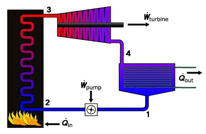
The Four Main Processes in the Rankine cycle :
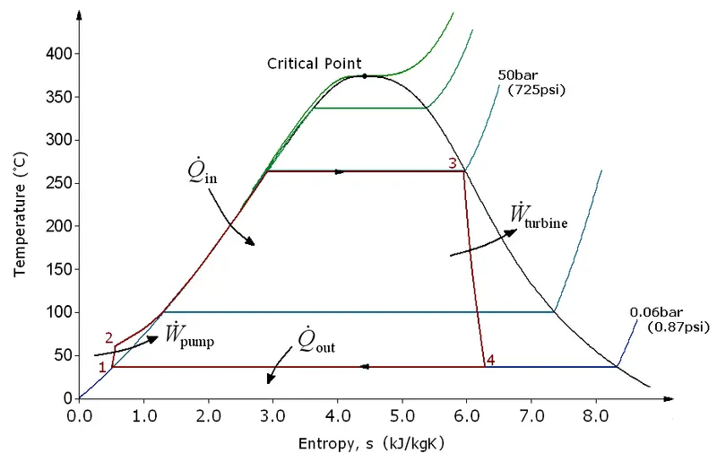
Process 1–2 : Isentropic Compression
In this process, the working fluid is pumped from low to high pressure with the help of a pump. As the fluid is a liquid at this stage, the pump requires little input energy. It is an isentropic process.
Process 2–3 : Constant Pressure Heat Addition
The high-pressure liquid enters a boiler, where it is heated at constant pressure by an external heat source to become a dry saturated vapour. The input energy required can be easily calculated graphically, using an enthalpy–entropy chart (h–s chart, or Mollier diagram), or numerically, using steam tables or software.
Process 3–4 : Isentropic Expansion
The dry saturated vapour expands through a turbine, generating power. This decreases the temperature and pressure of the vapour, and some condensation may occur. The output in this process can be easily calculated using the chart or tables noted above.
Process 4–1 : Constant pressure heat rejection
Then the wet vapour enters a condenser, where it is condensed at a constant pressure to become a saturated liquid.
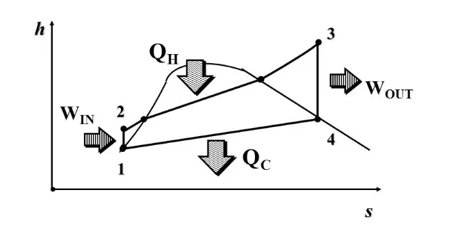
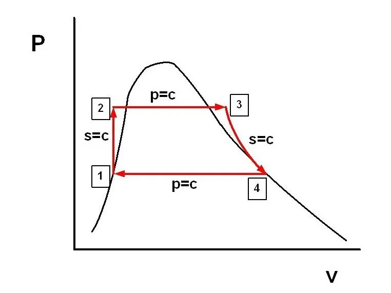
These processes can be represented as in the following diagrams -
i) T-s Diagram (Temperature vs Entropy)
ii) h-s Diagram(Enthalpy vs Entropy)
iii) P-v Diagram(Pressure vs Volume)
Equations for Rankine Cycle -
`Q_(In)= h_3-h_2`
`Q_(Out) = h_4-h_1`
`W_(P) = h_2-h_1`
`W_(T) = h_3-h_4`
`W_(Net) = W_T -W_P`
`eta_(therm) = W_(Net)/Q_(In)`
`bwr = Q_(In)/Q_(Out)`
`ssc = 3600/W_(Net)`
Where,
`h_1,h_2,h_3,h_4 =` Enthalpies at the state points 1,2,3,4 respectively
`Q_(In) =` Heat added or input to the system
`Q_(Out) =` Heat Rejected From the system
`W_(P) =` Work done by the Pump
`W_(T) =` Work done or got from the Turbine
`W_(Net) =` Net Work output from the System
`eta_(therm) =` Thermodynamic efficiency of the process (net power output per heat input)
`bwr =` Back Work Ratio (ratio of the compressor work to the turbine work)
`ssc =` Specific Steam Consumption (the steam consumed per unit output of power)
PROGRAM :
Consideration -
Considering State Points and Processes as mentioned below -
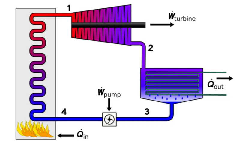
1-2 is Isentropic Expansion in Turbine
2-3 is Constant Pressure Heat Rejection by the Condenser
3-4 is Isentropic Compression in the Pump
4-1 is Constant Pressure Heat Addition by the boiler
Given -
In order to find state points and properties, a steam table function ' XSteam.m' was given for the use. The XSteam.m file is in following link -
https://drive.google.com/file/d/1RK_fvrOj38CIaQvmLT1S3daqHnxKCGU-/view
Given Required Inputs:
Turbine Inlet temperature = 400° C
Turbine Inlet Pressure = 30 bars
Turbine Outlet Pressure = 0.05 bars = Condenser Inlet Pressure
----------------------------------------------------------- PROGRAM ---------------------------------------------------------------
clear all;
close all;
clc;

% introduction display
fprintf('\t\t\t\t\t\t\t\t\t\t\t RANKINE CYCLE SIMULATOR \n');
fprintf('\n 1-2 is Isentropic Expansion in Turbine');
fprintf('\n 2-3 is Constant Pressure Heat Rejection by the Condenser');
fprintf('\n 3-4 is Isentropic Compression in the Pump');
fprintf('\n 4-1 is Constant Pressure Heat Addition by the boiler');


% Taking inputs from the user
p1 = input('\n n Enter the Inlet Pressure at the Turbine (in bar): ');
t1 = input('\n Enter the Inlet Temperature at the Turbine (in Degree Celcius): ');
p2 = input('\n Enter the Condenser Pressure/Turbine Outlet Pressure: ');

%-------- defining the State points and extracting data from the XSteam ------

% 1-2 Isentropic Expansion

h1 = XSteam('h_pT',p1,t1);      % Enthalpy at state pt. 1
s1 = XSteam('s_pT',p1,t1);      % Enthalpy at state pt. 1
tsat1 = XSteam('Tsat_p',p1);    % Saturation Temperature at p1
hf1 = XSteam('hL_p',p1);        % Enthalpy of Sat. liquid at p1
hg1 = XSteam('hV_p',p1);        % Enthalpy of Sat. vapour at p1
sf1 = XSteam('sL_p',p1);        % Entropy of Sat. liquid at p1
sg1 = XSteam('sV_p',p1);        % Entropy of Sat. vapour at p1

s2 = s1;                        % s2 is Entropy at state pt. 2
t2 = XSteam('T_ps',p2,s2);      % Temperature at state pt. 2
tsat2 = XSteam('Tsat_p',p2);    % Saturation Temperature at p2


% 2-3 Constant Pressure Heat Rejection

p3 = p2;                      % p3 is pressure at the inlet of the pump

hf2 = XSteam('hL_p',p2);      % Enthalpy of Sat. liquid at p2 at state pt. 3
hg2 = XSteam('hV_p',p2);      % Enthalpy of Sat. vapour at p2
sf3 = XSteam('sL_p',p3);      % Entropy of Sat. liquid at p2 at state pt.3
sg2 = XSteam('sV_p',p2);      % Entropy of sat. vapour at p2
hfg = hg2-hf2;
sfg = sg2-sf3;

if s2 > sg2
    x2 = 1;                  % x2 is the dryness fraction
    h2 = x2*hg2;             % Enthalpy at state pt. 2
else
    x2 = (s2-sf3)/sfg;
    h2 = hf2 + x2*hfg;
end

s3 = sf3;                   % Entropy at state pt. 3
h3 = hf2;                   % Enthalpy at state pt. 3

% 3-4 Isentropic Compression
s4 = s3;                    % Entropy at state pt. 4
t3 = tsat2;                 % temp. at state pt. 3

% 4-1 Constant Pressure Heat Addition
p4 = p1;
h4 = XSteam('h_ps',p4,s4);        % Enthalpy at state pt. 4
t4 = XSteam('T_ps',p4,s4);        % temp. at state pt. 4
%sf4 = XSteam('sL_p',p4);
%Ts4 = XSteam('Tsat_p',p4);
%CpL4 = XSteam('CpL_p',p4);
%t4 = Ts4/(exp((sf4-s4)/CpL4));

% 5 & 6 are Sub-State Points lies between process 4-1
h5 = XSteam('hL_p',p4);
t5 = XSteam('T_ph',p4,h5);
s5 = XSteam('s_ph',p4,h5);
h6 = XSteam('hV_p',p4);
t6 = XSteam('T_ph',p4,h6);
s6 = XSteam('s_ph',p4,h6);


% Work, Efficiency & Back Work Ratio Calculation

wt = h1-h2;         % Work out from the Turbine
wp = h4-h3;         % Work consumed by the pump

w = wt-wp;          % Net Work output of Rankine Cycle
qin = h1-h4;        % heat input
qout = h2-h3;       % heat rejected

eff = w/qin;        % Efficiency
eff_per = eff*100;  % Percentage Efficiency
bwr = wp/wt;        % Back Work Ratio
ssc = 3600/w;       % Specific Steam Consumption

% Display of results
fprintf('\n\n\t At State Point 1 \n');
fprintf('\t\t P1 = %.2f Bar \n',p1);
fprintf('\t\t T1 = %.2f Deg Celsius \n',t1);
fprintf('\t\t H1 = %.2f kJ/kg \n',h1);
fprintf('\t\t S1 = %.2f kJ/kgK ',s1);

fprintf('\n\n\t At State Point 2 \n');
fprintf('\t\t P2 = %.2f Bar \n',p2);
fprintf('\t\t T2 = %.2f Deg Celsius \n',t2);
fprintf('\t\t H2 = %.2f kJ/kg \n',h2);
fprintf('\t\t S2 = %.2f kJ/kgK \n',s2);
fprintf('\t\t X2 = %.2f ',x2);

fprintf('\n\n\t At State Point 3 \n');
fprintf('\t\t P3 = %.2f Bar \n',p3);
fprintf('\t\t T3 = %.2f Deg Celsius \n',t3);
fprintf('\t\t H3 = %.2f kJ/kg \n',h3);
fprintf('\t\t S3 = %.2f kJ/kgK ',s3);

fprintf('\n\n\t At State Point 4 \n');
fprintf('\t\t P4 = %.2f Bar \n',p4);
fprintf('\t\t T4 = %.2f Deg Celsius \n',t4);
fprintf('\t\t H4 = %.2f kJ/kg \n',h4);
fprintf('\t\t S4 = %.2f kJ/kgK ',s4);

fprintf('\n\n\t Work Done by Turbine(Wt) = %.2f kJ/kg \n',wt);
fprintf('\t Work Consumed by Pump(Wp) = %.2f kJ/kg',wp);

fprintf('\n\n\t Net Work Done(W) = %.2f kJ/kg \n',w);
fprintf('\t Efficiency of the Cycle(Ntherm) = %.2f %% \n',eff_per);
fprintf('\t Back Work Ratio = %f \n',bwr);
fprintf('\t Specific Steam Consumption(S.S.C) = %.2f kg/kWh \n',ssc);

%-----------------------------------   Plotting Graphs   -----------------------------------

% For saturation lines
p = 0.01:0.01:400;
for i = 1:length(p)
    t(i) = XSteam('Tsat_p',p(i));
    sf(i) = XSteam('sL_T',p(i));
    sg(i) = XSteam('sV_T',p(i));
    hf(i) = XSteam('hL_T',p(i));
    hg(i) = XSteam('hV_T',p(i));
end

%  Plotting T-S Diagram
figure(1)
hold on;

% Saturation Lines
plot(sf,p,':','color','k','linewidth',2);
plot(sg,p,':','color','k','linewidth',2);

% 1-2 Isentropic Expansion
plot([s1 s2],[t1 t2],'g','linewidth',2);

% 2-3 Constant Pressure Heat Rejection
if x2<1
    plot([s2 s3],[t2 t3],'b','linewidth',2);
else
    sh2 = linspace(sg2,s2,100);                 % sh2 is the entropies when the state pt. 2 lies in superheat region
    for j = 1:length(sh2)
        th2(j) = XSteam('T_ps',p2,sh2(j));      % th2 is the temperature corresponding to sh2
    end
    plot(sh2,th2,'b','linewidth',2);
    plot([sg2 s3],[tsat2 t3],'b','linewidth',2);
end

% 3-4 Isentropic Compression
plot([s3 s4],[t3 t4],'m','linewidth',2);

% 4-1 Constant Pressure Heat Addition
sc4 = linspace(s4,s5,500);                     % sc4 is used to get entropies from the state pt. 4 - 5, which lies in sub-cooled region
    for j = 1:length(sc4)
        tc4(j) = XSteam('T_ps',p4,sc4(j));     % tc4 is the temperature corresponding to sc4
    end
plot(sc4,tc4,'r','linewidth',2);

plot([s5 s6],[t5 t6],'r','linewidth',2);

sh1 = linspace(s6,s1,500);                     % sh1 is used to get entropies from the state pt. 6 - 1, which lies in superheat region
    for j = 1:length(sh1)
        th1(j) = XSteam('T_ps',p4,sh1(j));     % th1 is the temperature corresponding to sh1
    end
plot(sh1,th1,'r','linewidth',2);

title('Temperature vs Entropy');
xlabel('Entropy (in kJ/kgK)');  ylabel('Temperature (in Deg Celcius)');
legend('Sat. Liquid Line','Sat. Vapour Line','1-2 Isentropic Compression','2-3 Constant Pressure Heat Rejection'...
    ,'3-4 Isentropic Compression','4-1 Constant Pressure Heat Addition','Location','northwest');

% plotting State points
text(s1+0.1,t1+10,'1');
text(s2+0.1,t2,'2');
text(s3+0.15,t3-10,'3');
text(s4-0.15,t4+10,'4');
text(s5-0.15,t5+10,'5');
text(s6-0.15,t6+10,'6');
grid on;

hold off;


%  Plotting H-S Diagram
figure(2)
hold on;

% Saturation Lines
plot(sf,hf,':','color','k','linewidth',2);
plot(sg,hg,':','color','k','linewidth',2);

% 1-2 Isentropic Expansion
plot([s1 s2],[h1 h2],'g','linewidth',2);

% 2-3 Constant Pressure Heat Rejection
plot([s2 s3],[h2 h3],'b','linewidth',2);

% 3-4 Isentropic Compression
plot([s3 s4],[h3 h4],'m','linewidth',2);

% 4-1 Constant Pressure Heat Addition
sc4 = linspace(s4,s5,500);                     % sc4 is used to get entropies from the state pt. 4 - 5, which lies in sub-cooled region
    for j = 1:length(sc4)
        hc4(j) = XSteam('h_ps',p4,sc4(j));     % hc4 is the enthalpy corresponding to sc4
    end
plot(sc4,hc4,'r','linewidth',2);

plot([s5 s6],[h5 h6],'r','linewidth',2);

hsh1 = linspace(h6,h1,500);                    % hsh1 is used to get enthalpies from the state pt. 6 - 1, which lies in superheat region
    for j = 1:length(sh1)
        ssh1(j) = XSteam('s_ph',p4,hsh1(j));   % ssh1 is the temperature corresponding to hsh1
    end
plot(ssh1,hsh1,'r','linewidth',2);

title('Enthalpy vs Entropy');
xlabel('Entropy (in kJ/kgK)');  ylabel('Enthalpy (in kJ/kg)');
legend('Sat. Liquid Line','Sat. Vapour Line','1-2 Isentropic Compression','2-3 Constant Pressure Heat Rejection'...
    ,'3-4 Isentropic Compression','4-1 Constant Pressure Heat Addition','Location','northwest');

% plotting State points
text(s1+0.1,h1+10,'1');
text(s2+0.1,h2,'2');
text(s3+0.15,h3-10,'3');
text(s4-0.15,h4+10,'4');
text(s5-0.15,h5+10,'5');
text(s6-0.15,h6+10,'6');
grid on;
hold off;
CODING EXPLANATION :
1. Here, we have used input() function in order to take the values of the parameter from the user, and these received values are stored in respective variables.
% Taking inputs from the user
p1 = input('\n \n Enter the Inlet Pressure at the Turbine (in bar): ');
t1 = input('\n Enter the Inlet Temperature at the Turbine (in Degree Celcius): ');
p2 = input('\n Enter the Condenser Pressure/Turbine Outlet Pressure: ');
2. In this, the getting parameters and properties at the state points using the function 'XSteam.m'. Then we have made the if-else for the two cases of possibility for the dryness fraction(x) one state point lying in the fluid-vapour region and second lying the superheat region.
% 1-2 Isentropic Expansion

h1 = XSteam('h_pT',p1,t1);      % Enthalpy at state pt. 1
s1 = XSteam('s_pT',p1,t1);      % Enthalpy at state pt. 1
tsat1 = XSteam('Tsat_p',p1);    % Saturation Temperature at p1
hf1 = XSteam('hL_p',p1);        % Enthalpy of Sat. liquid at p1
hg1 = XSteam('hV_p',p1);        % Enthalpy of Sat. vapour at p1
sf1 = XSteam('sL_p',p1);        % Entropy of Sat. liquid at p1
sg1 = XSteam('sV_p',p1);        % Entropy of Sat. vapour at p1

s2 = s1;                        % s2 is Entropy at state pt. 2
t2 = XSteam('T_ps',p2,s2);      % Temperature at state pt. 2
tsat2 = XSteam('Tsat_p',p2);    % Saturation Temperature at p2


% 2-3 Constant Pressure Heat Rejection

p3 = p2;                      % p3 is pressure at the inlet of the pump

hf2 = XSteam('hL_p',p2);      % Enthalpy of Sat. liquid at p2 at state pt. 3
hg2 = XSteam('hV_p',p2);      % Enthalpy of Sat. vapour at p2
sf3 = XSteam('sL_p',p3);      % Entropy of Sat. liquid at p2 at state pt.3
sg2 = XSteam('sV_p',p2);      % Entropy of sat. vapour at p2
hfg = hg2-hf2;
sfg = sg2-sf3;

if s2 > sg2
    x2 = 1;                  % x2 is the dryness fraction
    h2 = x2*hg2;             % Enthalpy at state pt. 2
else
    x2 = (s2-sf3)/sfg;
    h2 = hf2 + x2*hfg;
end

s3 = sf3;                   % Entropy at state pt. 3
h3 = hf2;                   % Enthalpy at state pt. 3

% 3-4 Isentropic Compression
s4 = s3;                    % Entropy at state pt. 4
t3 = tsat2;                 % temp. at state pt. 3

% 4-1 Constant Pressure Heat Addition
p4 = p1;
h4 = XSteam('h_ps',p4,s4);        % Enthalpy at state pt. 4
t4 = XSteam('T_ps',p4,s4);        % temp. at state pt. 4
3. Assigning and calculating the sub-state points(i.e. 5 & 6) between the process 4-1 at the saturation liquid line and saturated vapour line.
% 5 & 6 are Sub-State Points lies between process 4-1
h5 = XSteam('hL_p',p4);
t5 = XSteam('T_ph',p4,h5);
s5 = XSteam('s_ph',p4,h5);
h6 = XSteam('hV_p',p4);
t6 = XSteam('T_ph',p4,h6);
s6 = XSteam('s_ph',p4,h6);
4. Calculating the efficiency, work done, etc and other characteristic parameters of the Rankine cycle using their respective Equations.
% Work, Efficiency & Back Work Ratio Calculation

wt = h1-h2;         % Work out from the Turbine
wp = h4-h3;         % Work consumed by the pump

w = wt-wp;          % Net Work output of Rankine Cycle
qin = h1-h4;        % heat input
qout = h2-h3;       % heat rejected

eff = w/qin;        % Efficiency
eff_per = eff*100;  % Percentage Efficiency
bwr = wp/wt;        % Back Work Ratio
ssc = 3600/w;       % Specific Steam Consumption
5. Plotting T-s and h-s Diagram. Here we have taken data from the XSteam.m function file in-order to plot the saturation lines. Also, the state pt. 4 lies in the sub-cooled region so, from that point to the saturation line the path line is not linear therefore in-order to plot that we have to get the data parameter of the points between them. Similar method is used to plot the path between sat. line to the state pt.1 which lies in the superheat region. And same for the state pt. 2 a case situation is defined if the state point is in the fluid-vapour region then the path line is straight or if the point lies outside at the superheat region the same method is used told above to plot. the pathlines in the Liquid-Vapour region is always straight.
% For saturation lines
p = 0.01:0.01:400;
for i = 1:length(p)
    t(i) = XSteam('Tsat_p',p(i));
    sf(i) = XSteam('sL_T',p(i));
    sg(i) = XSteam('sV_T',p(i));
    hf(i) = XSteam('hL_T',p(i));
    hg(i) = XSteam('hV_T',p(i));
end

%  Plotting T-S Diagram
figure(1)
hold on;

% Saturation Lines
plot(sf,p,':','color','k','linewidth',2);
plot(sg,p,':','color','k','linewidth',2);

% 1-2 Isentropic Expansion
plot([s1 s2],[t1 t2],'g','linewidth',2);

% 2-3 Constant Pressure Heat Rejection
if x2<1
    plot([s2 s3],[t2 t3],'b','linewidth',2);
else
    sh2 = linspace(sg2,s2,100);                 % sh2 is the entropies when the state pt. 2 lies in superheat region
    for j = 1:length(sh2)
        th2(j) = XSteam('T_ps',p2,sh2(j));      % th2 is the temperature corresponding to sh2
    end
    plot(sh2,th2,'b','linewidth',2);
    plot([sg2 s3],[tsat2 t3],'b','linewidth',2);
end

% 3-4 Isentropic Compression
plot([s3 s4],[t3 t4],'m','linewidth',2);

% 4-1 Constant Pressure Heat Addition
sc4 = linspace(s4,s5,500);                     % sc4 is used to get entropies from the state pt. 4 - 5, which lies in sub-cooled region
    for j = 1:length(sc4)
        tc4(j) = XSteam('T_ps',p4,sc4(j));     % tc4 is the temperature corresponding to sc4
    end
plot(sc4,tc4,'r','linewidth',2);

plot([s5 s6],[t5 t6],'r','linewidth',2);

sh1 = linspace(s6,s1,500);                     % sh1 is used to get entropies from the state pt. 6 - 1, which lies in superheat region
    for j = 1:length(sh1)
        th1(j) = XSteam('T_ps',p4,sh1(j));     % th1 is the temperature corresponding to sh1
    end
plot(sh1,th1,'r','linewidth',2);

title('Temperature vs Entropy');
xlabel('Entropy (in kJ/kgK)');  ylabel('Temperature (in Deg Celcius)');
legend('Sat. Liquid Line','Sat. Vapour Line','1-2 Isentropic Compression','2-3 Constant Pressure Heat Rejection'...
    ,'3-4 Isentropic Compression','4-1 Constant Pressure Heat Addition','Location','northwest');

text(s1+0.1,t1+10,'1');
text(s2+0.1,t2,'2');
text(s3+0.15,t3-10,'3');
text(s4-0.15,t4+10,'4');
text(s5-0.15,t5+10,'5');
text(s6-0.15,t6+10,'6');
grid on;

hold off;


%  Plotting H-S Diagram
figure(2)
hold on;

% Saturation Lines
plot(sf,hf,':','color','k','linewidth',2);
plot(sg,hg,':','color','k','linewidth',2);

% 1-2 Isentropic Expansion
plot([s1 s2],[h1 h2],'g','linewidth',2);

% 2-3 Constant Pressure Heat Rejection
plot([s2 s3],[h2 h3],'b','linewidth',2);

% 3-4 Isentropic Compression
plot([s3 s4],[h3 h4],'m','linewidth',2);

% 4-1 Constant Pressure Heat Addition
sc4 = linspace(s4,s5,500);                     % sc4 is used to get entropies from the state pt. 4 - 5, which lies in sub-cooled region
    for j = 1:length(sc4)
        hc4(j) = XSteam('h_ps',p4,sc4(j));     % hc4 is the enthalpy corresponding to sc4
    end
plot(sc4,hc4,'r','linewidth',2);

plot([s5 s6],[h5 h6],'r','linewidth',2);

hsh1 = linspace(h6,h1,500);                    % hsh1 is used to get enthalpies from the state pt. 6 - 1, which lies in superheat region
    for j = 1:length(sh1)
        ssh1(j) = XSteam('s_ph',p4,hsh1(j));   % ssh1 is the temperature corresponding to hsh1
    end
plot(ssh1,hsh1,'r','linewidth',2);

title('Enthalpy vs Entropy');
xlabel('Entropy (in kJ/kgK)');  ylabel('Enthalpy (in kJ/kg)');
legend('Sat. Liquid Line','Sat. Vapour Line','1-2 Isentropic Compression','2-3 Constant Pressure Heat Rejection'...
    ,'3-4 Isentropic Compression','4-1 Constant Pressure Heat Addition','Location','northwest');

text(s1+0.1,h1+10,'1');
text(s2+0.1,h2,'2');
text(s3+0.15,h3-10,'3');
text(s4-0.15,h4+10,'4');
text(s5-0.15,h5+10,'5');
text(s6-0.15,h6+10,'6');
grid on;
hold off;
OUTPUT :
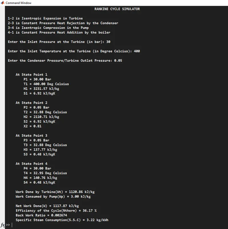
T-s Diagram -
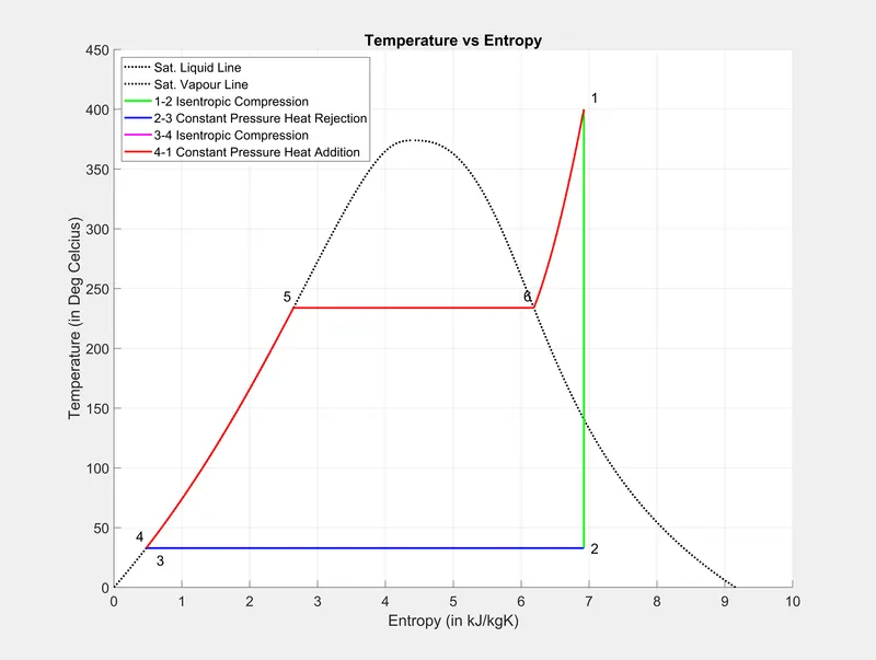
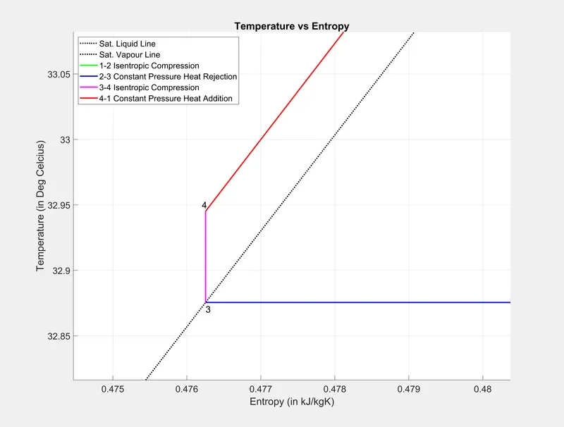
h-s Diagram -
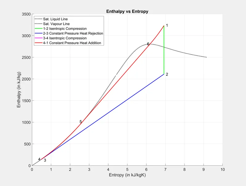
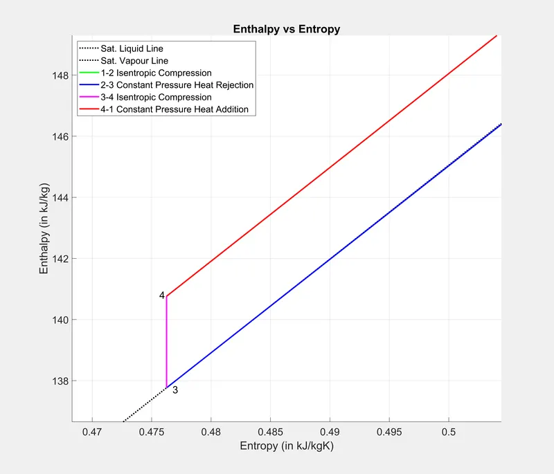
ERRORS OCCURED :
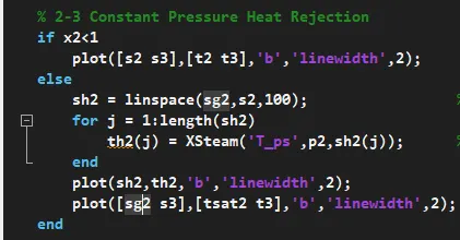
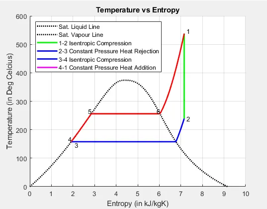
A logical error was faced while plotting for the condition at which the state point lies on superheat region, for the inputs of P1= 44 bar, T1 = 538 deg. celsius, and p2 = 5.83 bar.
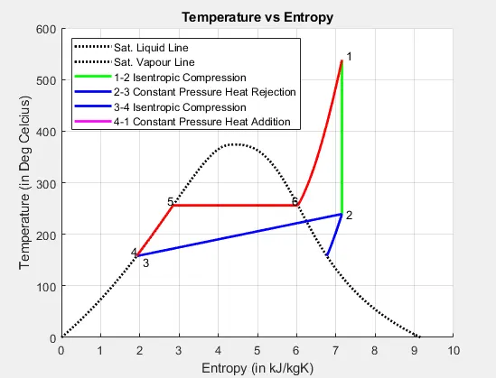
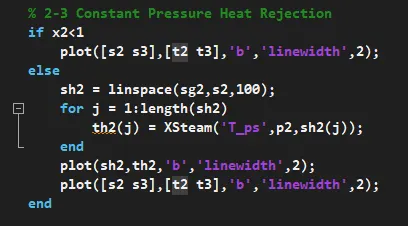
The error was solved with the following code -
REFERENCE :
https://en.wikipedia.org/wiki/Rankine_cycle
https://www.thermopedia.com/content/1072/#RANKINE_CYCLE_FIG1
http://www.expertsmind.com/topic/vapor-power-cycles/rankine-cycle-97680.aspx
For Result Verification -
https://sites.google.com/a/learncheme.com/learncheme-modules/rankine-cycle/example-problems