Week 3 - External flow simulation over an Ahmed body.

AIM : To perform Simulation of Flow over a Ahmed Body.

OBJECTIVES : 

• Setting up the Geometry in Spaceclaim.
• Create optimal meshing for the model in Ansys Mesher.
• Setup the model for the analysis from the given data.
• Run the simulation and Post Process the results.
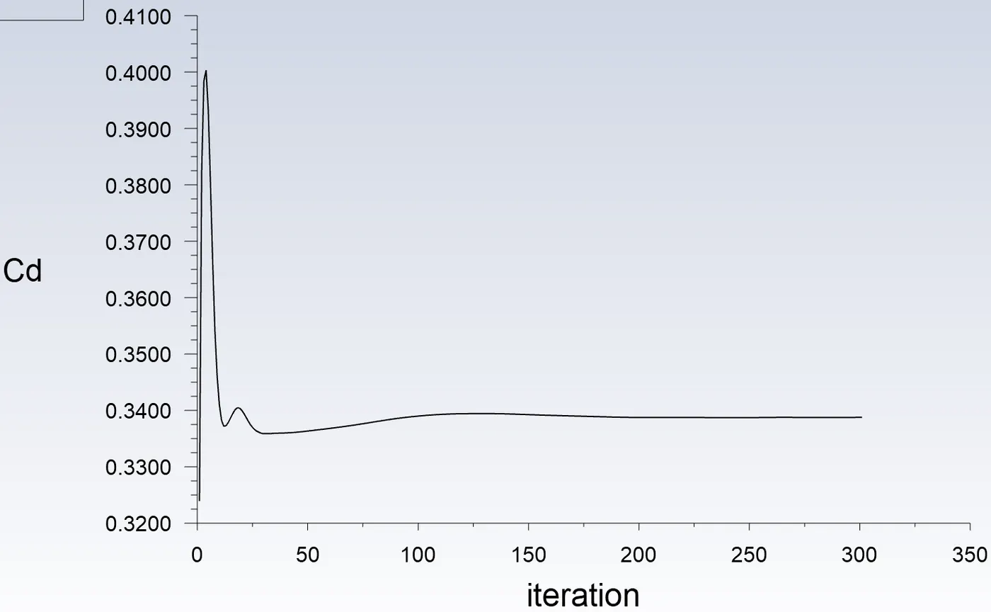
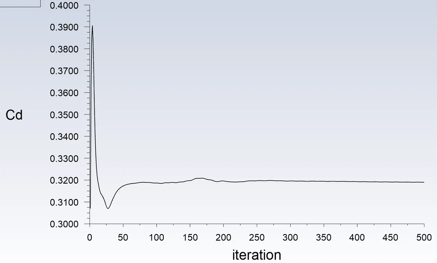
• Get Results for velocity of 25m/sec, the drag coefficient should be around 0.33.
• Do analysis for different levels of mesh refinement and use of inflation layer.
• Perform the grid independency test and provide the values of drag and lift with each case. 
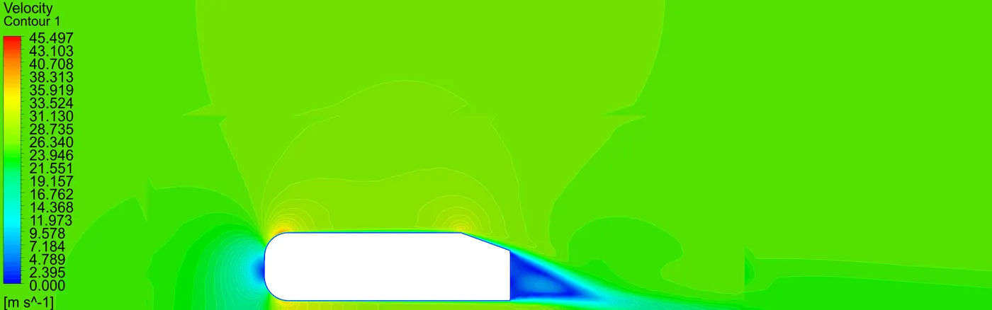
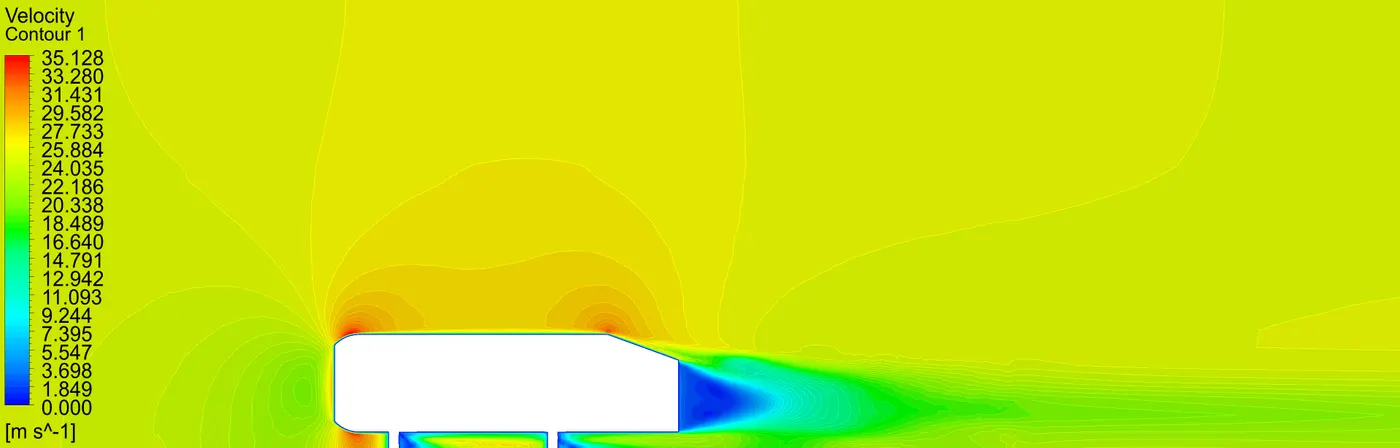
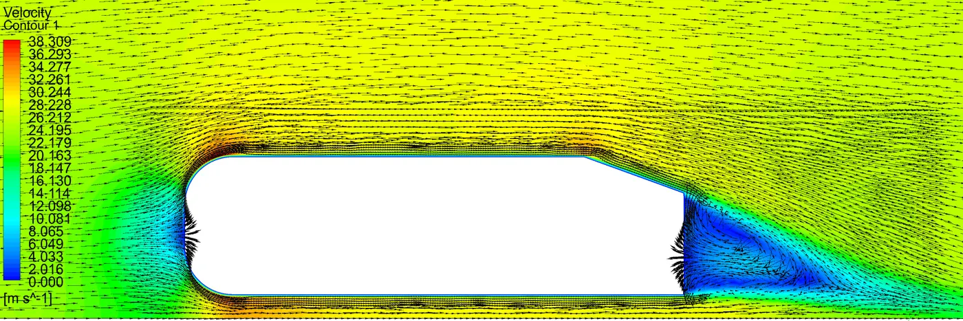
• The vector plot clearly showing the wake region. 

INTRODUCTION :

The Ahmed body represents a simplified, ground vehicle geometry of a bluff body type. Its shape is simple enough to allow for accurate flow simulation but retains some important practical features relevant to automobile bodies. The geometry was first defined by Ahmed, who also measured its aerodynamic properties in wind-tunnel experiments. Further experiments have also been performed by Lienhart and Becker.

Although it has a very simple shape, Ahmed body allows us to capture characteristic features that are relevant to bodies in the automobile industry. This model is also used to describe the turbulent flow field around a car-like geometry. Once the numerical model in validated, it is used to design new models of the car. Car companies makes numerous attempts to develop modified designs to effectively reduce the aerodynamic drag force which occurs at the rear end without putting any constraints in the stability, comfort and safety of the passengers.

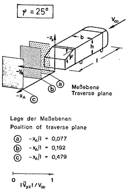
Following is the Ahmed Body geometry by S.R. Ahmed, [Ref.1]

 

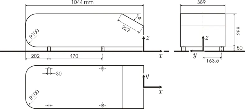
For our case the `phi =25^@`

STEPS / PROCEDURE :

1) Geometry 

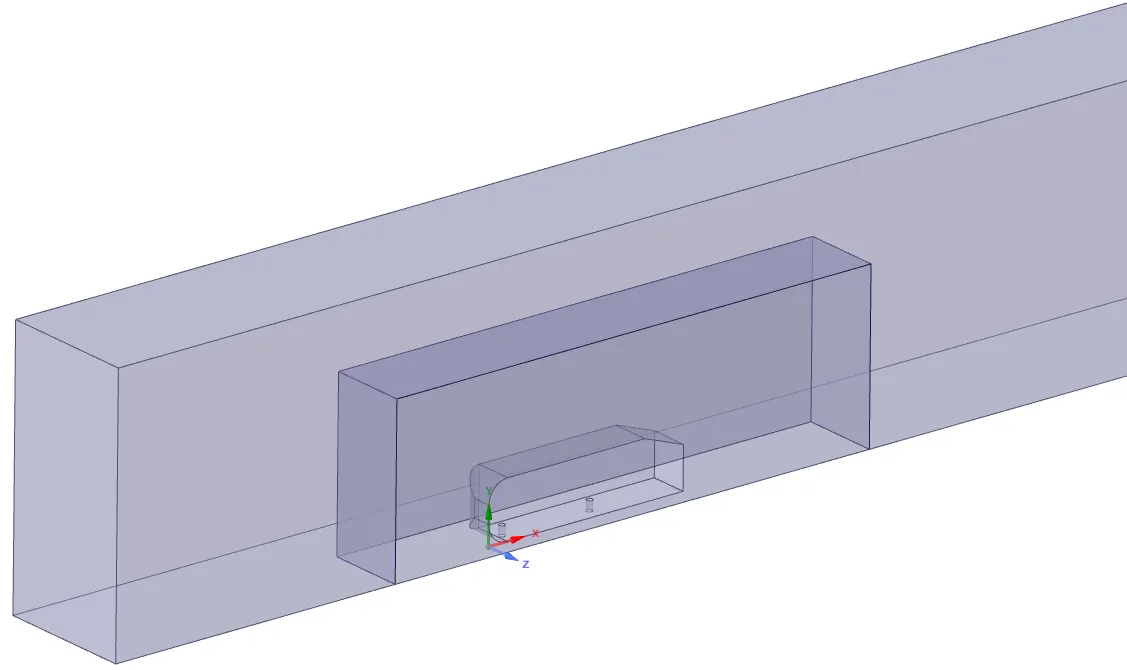
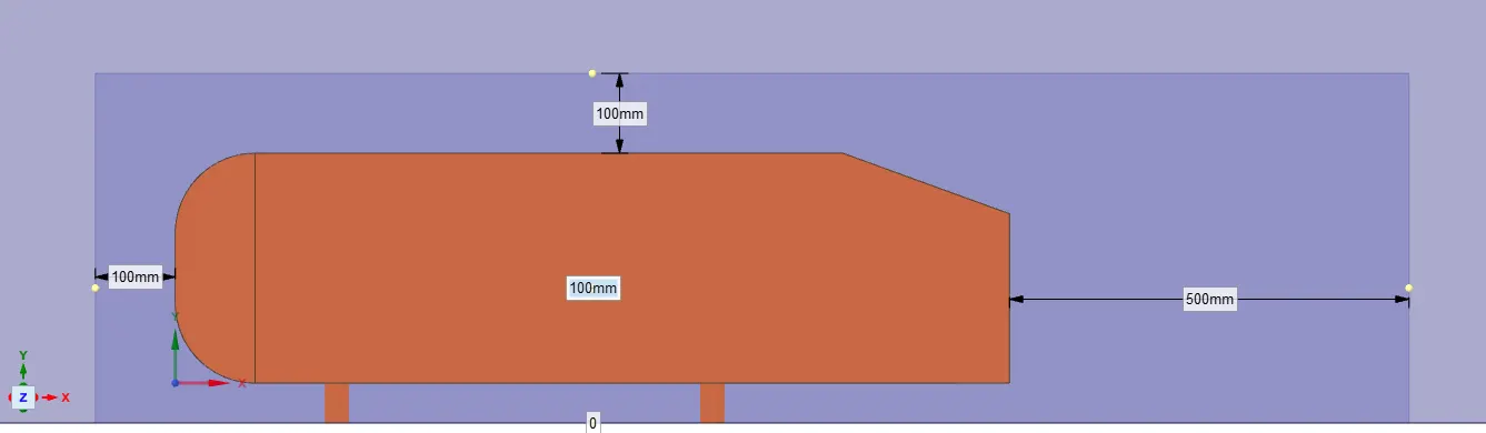
The Following is the geometry based on given Step file & dimensions in spaceclaim -

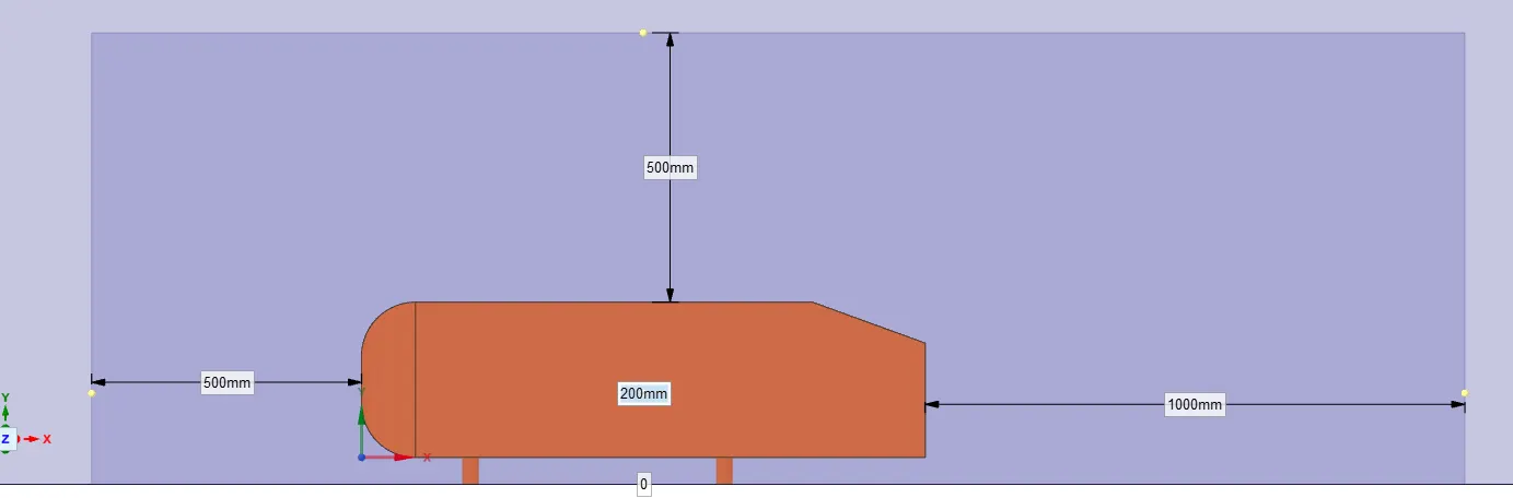
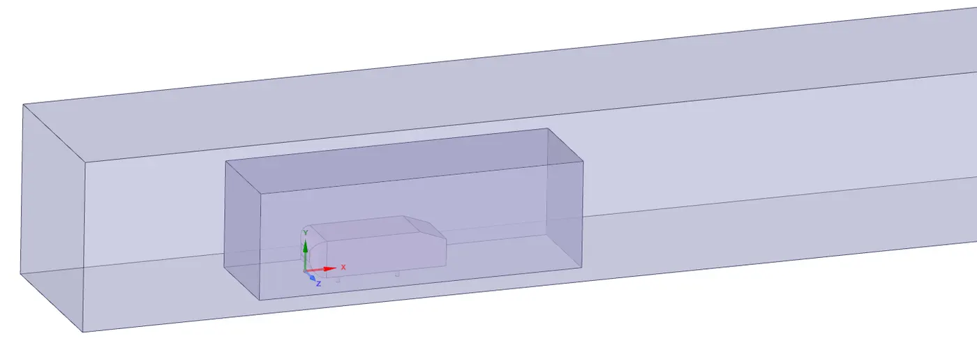
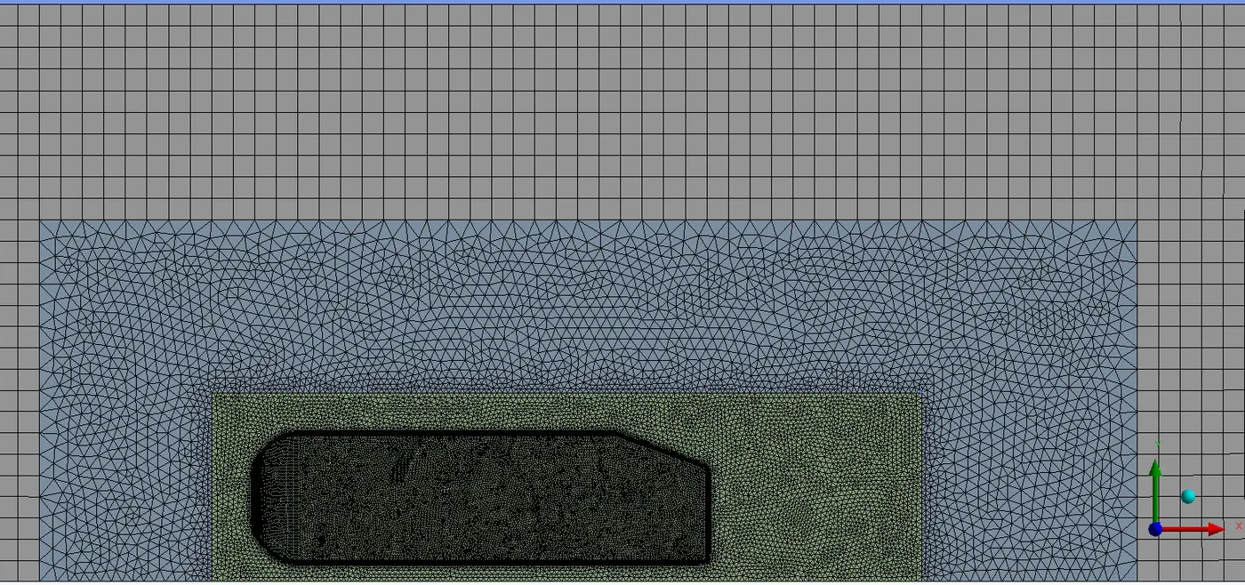
As the body is perfectly symmetric, we can simulate by considering only half the body. This is the best practice where we can save on the number of cells and get the results faster as well. 

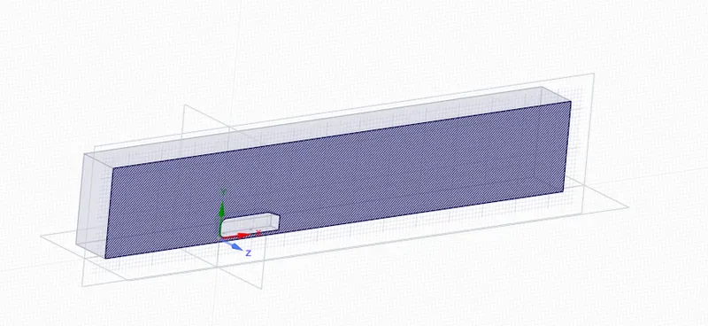
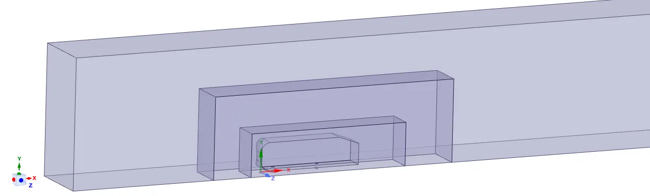
For the 3rd Refinement, created 1 more inner zone for more refinement.

 

2) Meshing

After doing Geometry preparation, we gone open the geometry in Ansys Mesher via workbench -

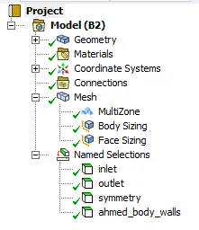
• Creating Named Selections
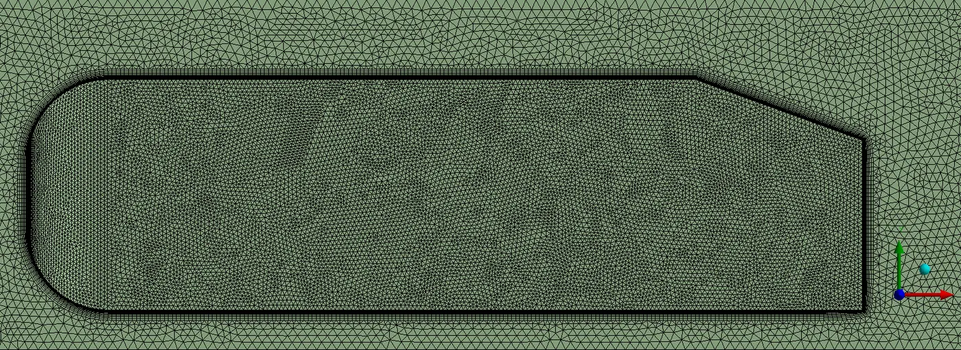
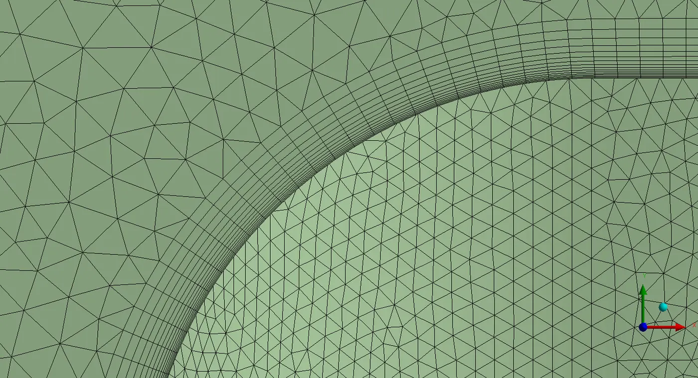
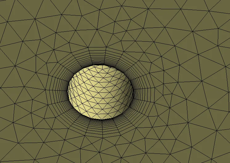
• Assigning proper mesh sizing
• Creating Inflation layers at the surrounding of the cylinder wall
• Checkng mesh quality.

             

   

      

                                

      

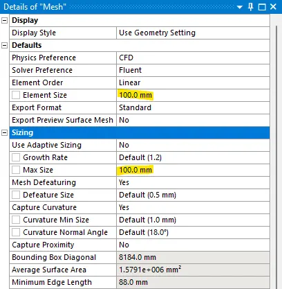
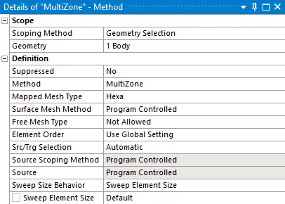
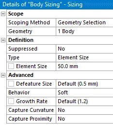
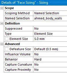
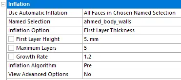
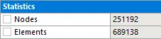
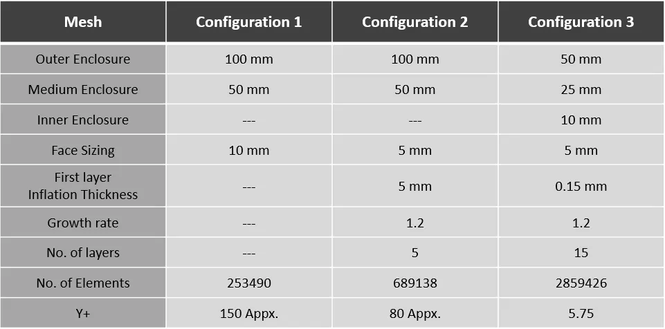
 Mesh Quality Verification-

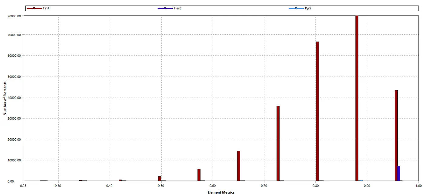
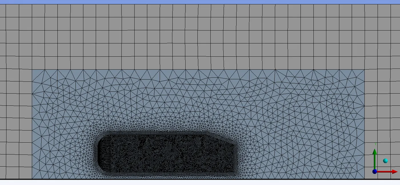
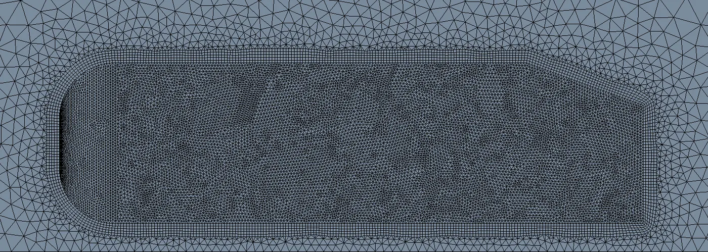
Following is the surface mesh And Element quality of the Case Setup -

 i) For Mesh Configuration 1 -

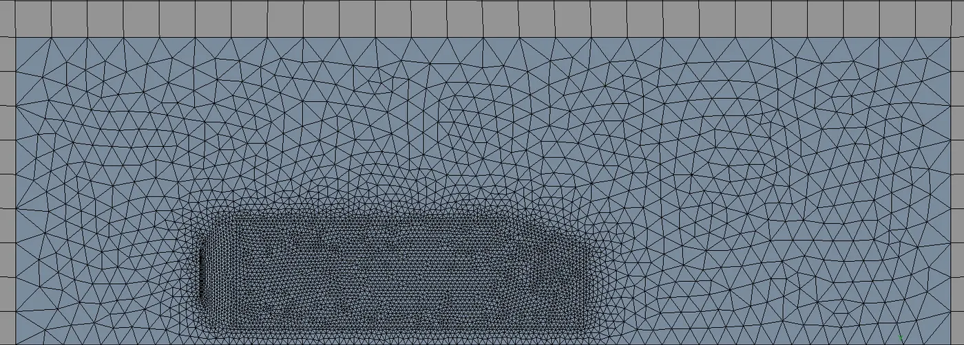
 ii) For Mesh Configuration 2 -

 

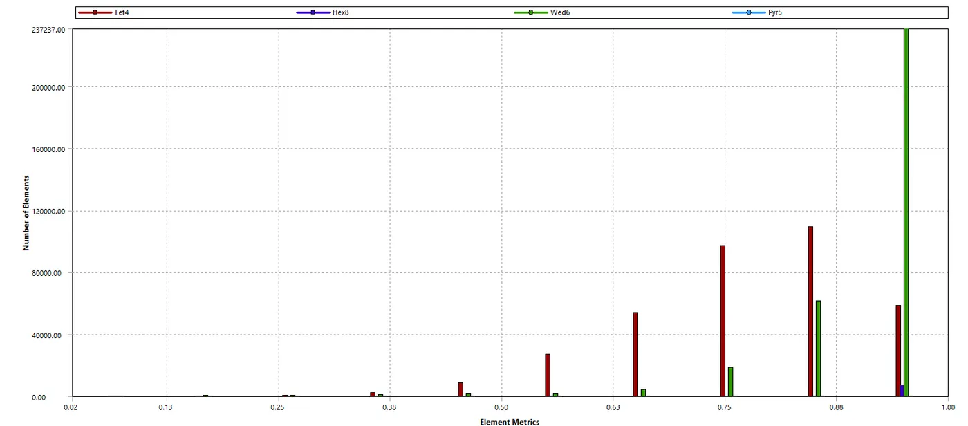
 iii) For Mesh Configuration 3 -

 

 

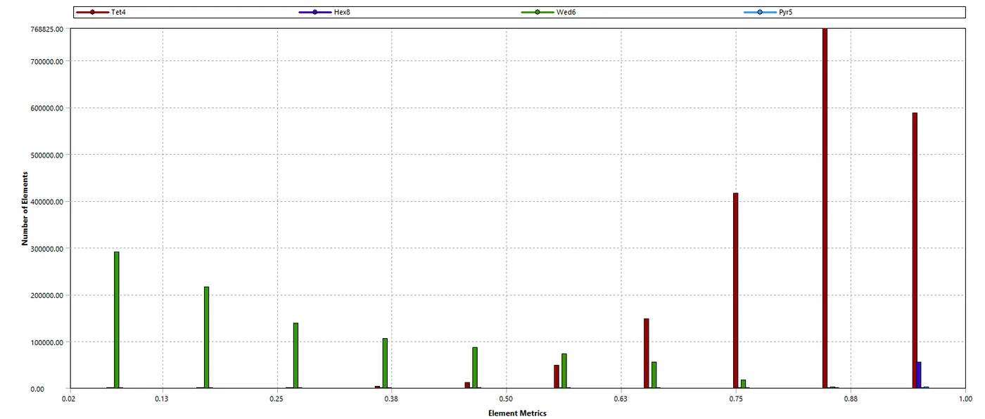
We can the mesh quality is very satisfied. 90% of the mesh cell are lying on good quality range. 

3) Solver Settings -

Closing the Mesher & opening the Fluent Solver from the workbench

Checking the the Double precision option and selecting no. of parallel process.

Setting solver settings and initialization values.

Since the velocity has been decided to be 25m/s and the speed of sound at sea level is 340.197m/s.

Then, the mach number will be = `(25*ms^(-1))/(340.197*ms^(-1))`

Therefore, the mach number is lesser than 0.3, hence a pressure based solver must be used.

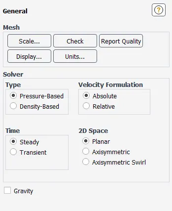
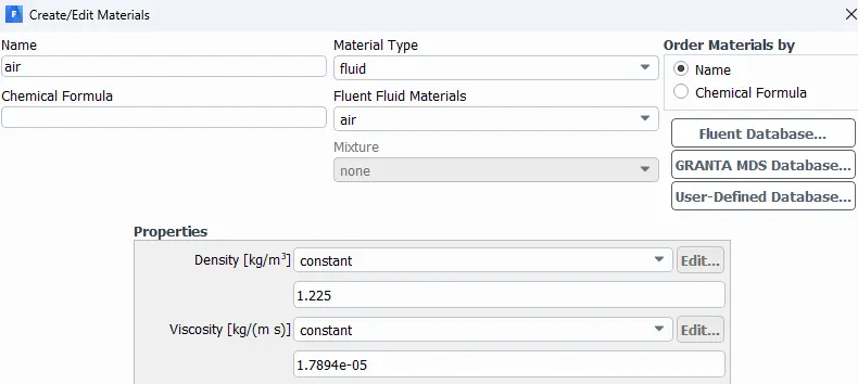
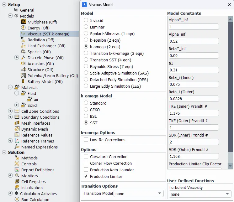
Selecting the turbulence model and its settings.

Now assigning the boundary conditions inlets, outlet, and walls.

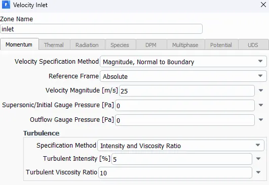
And oultet is set to - Pressure Outlet

Body walls - No-slip wall

Rest of the boundary is set to - Symmetry

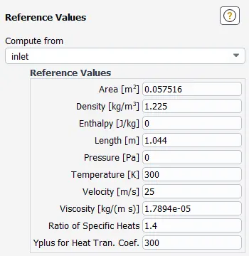
Reference Values for the Solution should computed from the inlet after assigning all properties and Boundary conditions.

Setting Inilization, here we are using Hybrid Initialization.

Creating Solution reports.

   

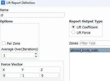
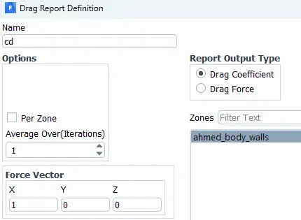
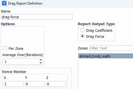
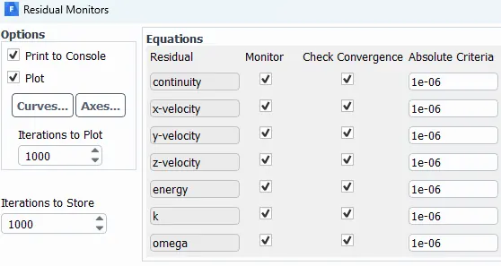
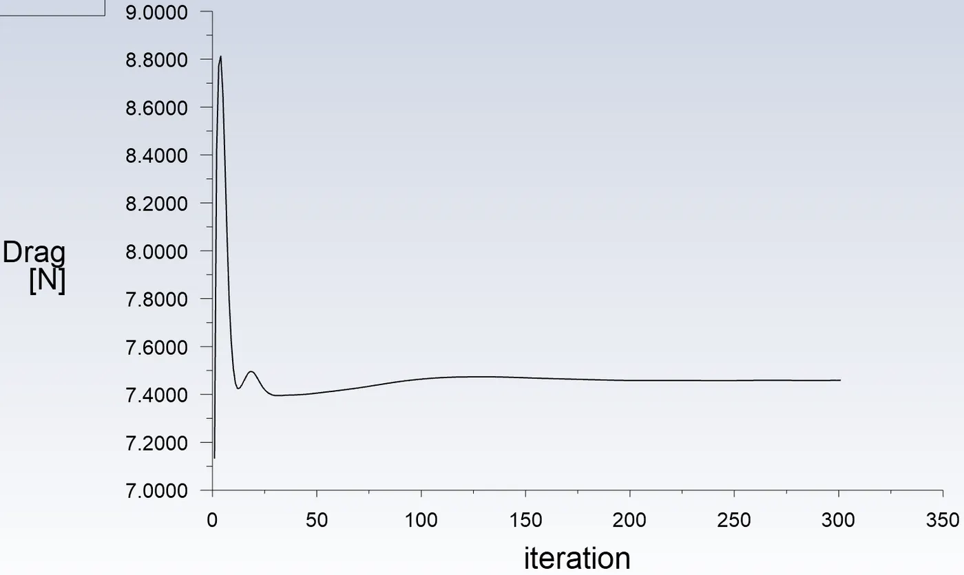
The convergence criteria has been turned off since we have monitor flow with respect to time.

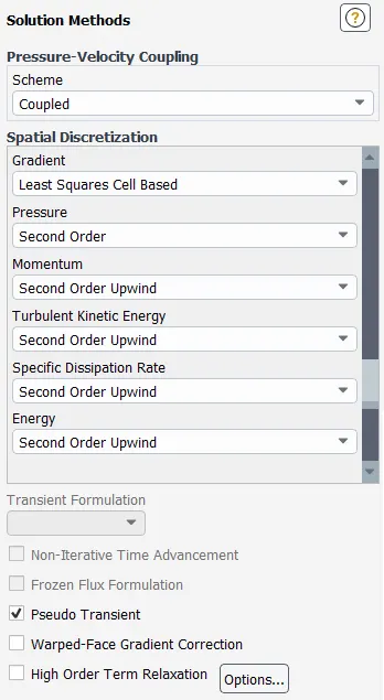
Keeping the Solution method & discretization schemes as shown below.

  

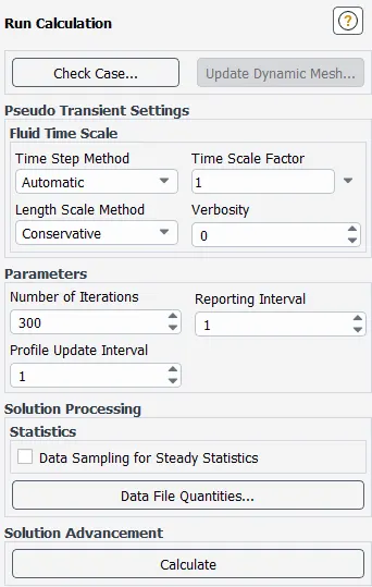
For Mesh Configuration 1, we perform 2 simulations one withK-epsilon and one with k-omega SST turbulence model.

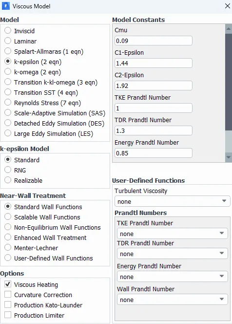
Rest of the settings will be same.

Now there will be 4 cases to analyse -

1) Mesh Config. 1 with k-Epsilon

2) Mesh Config. 1 with k-Omega SST

3) Mesh Config. 2 with k-Omega SST

4) Mesh Config. 3 with k-Omega SST

POST PROCESSING :

Outputs

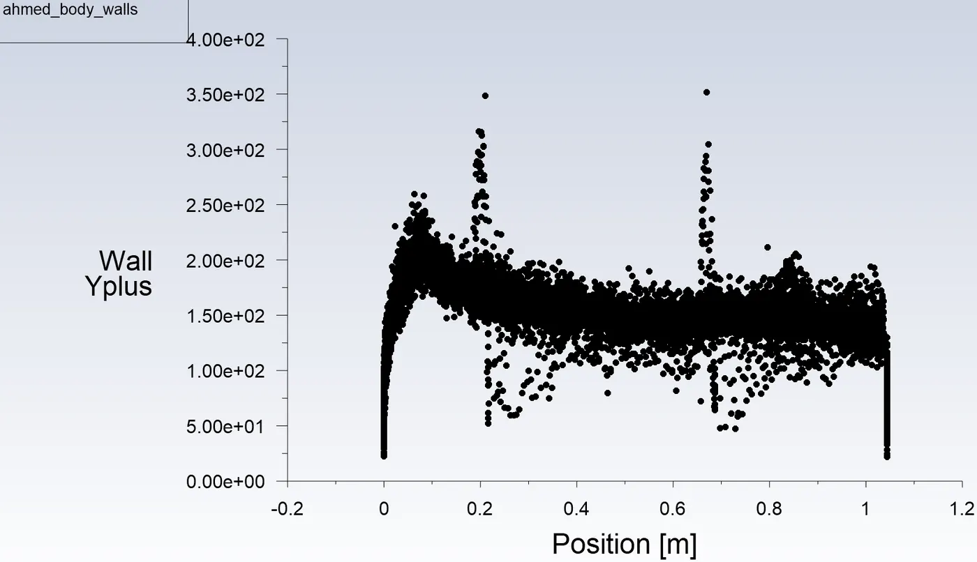
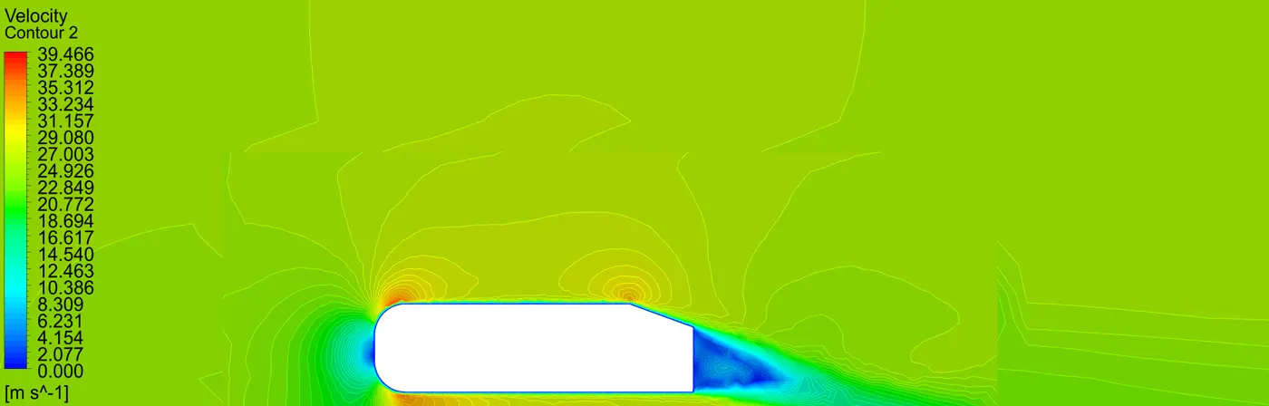
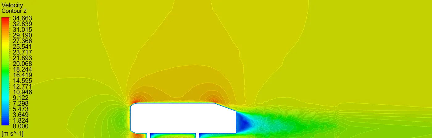
1. For Mesh Config. 1 with k-Epsilon -

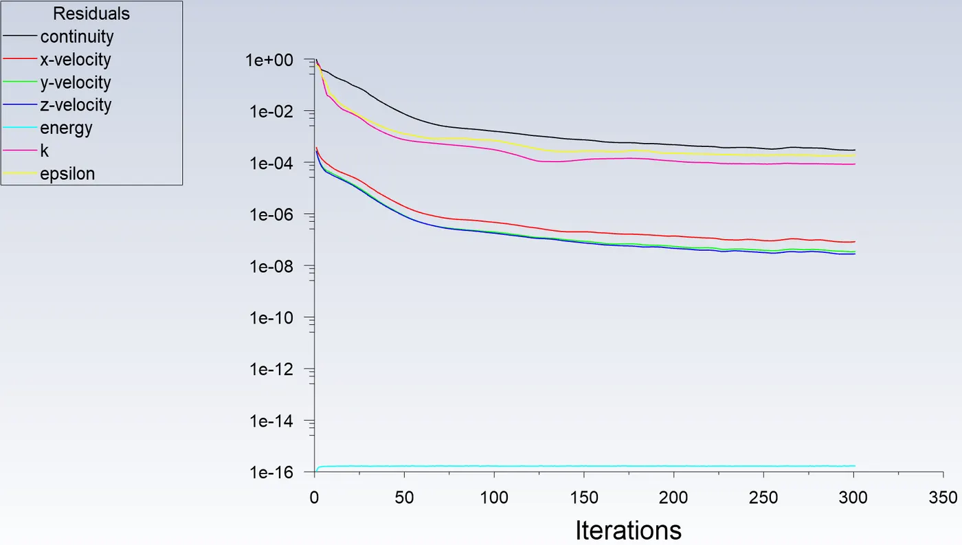
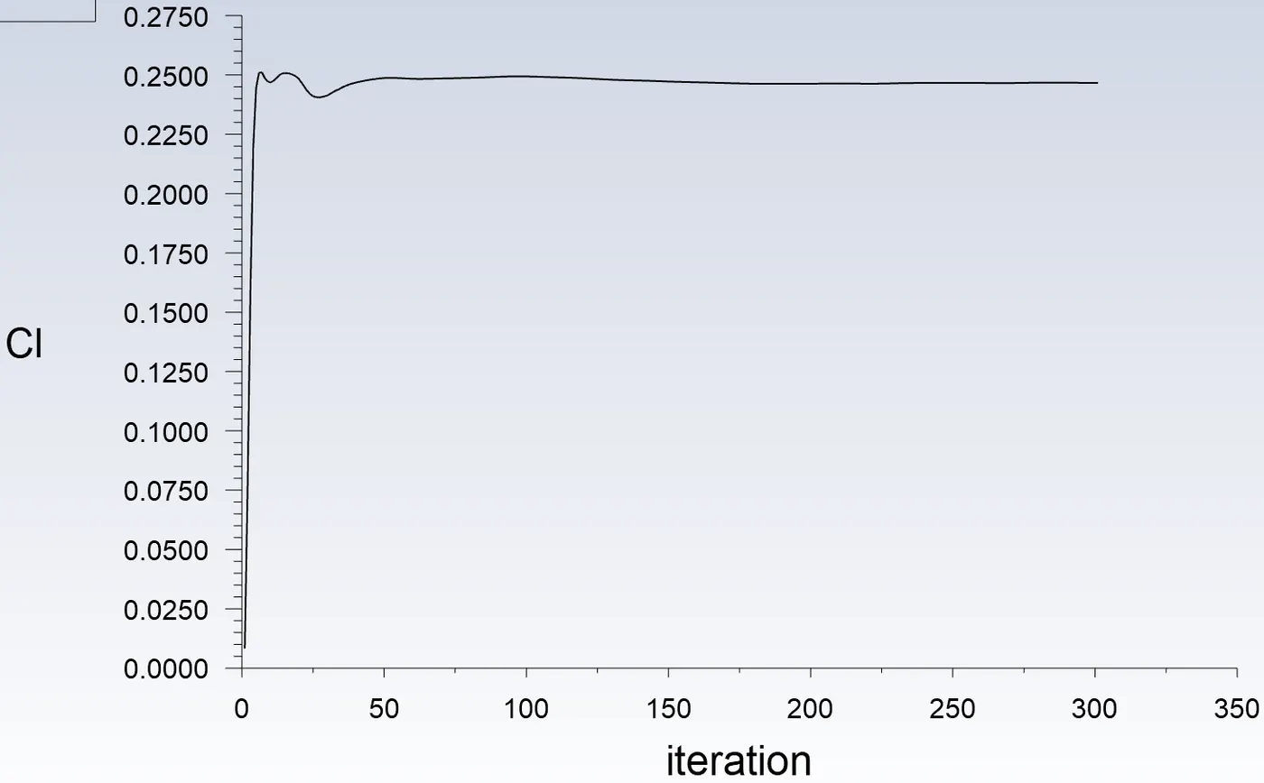
      Residuals and Solution Plot -

          

          

          

          

          

     Contour Plots -

          Velocity Contour -

          

          

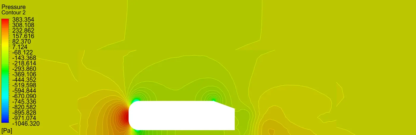
          Pressure Contour - 

          

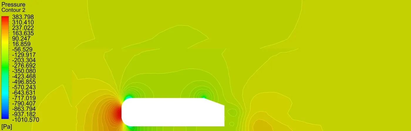
2. For Mesh Config. 1 with k-Omega SST -

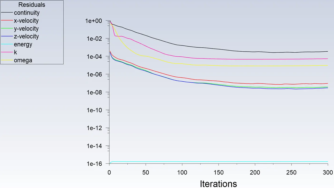
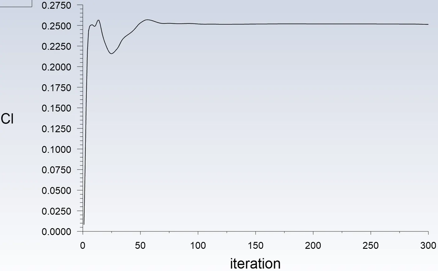
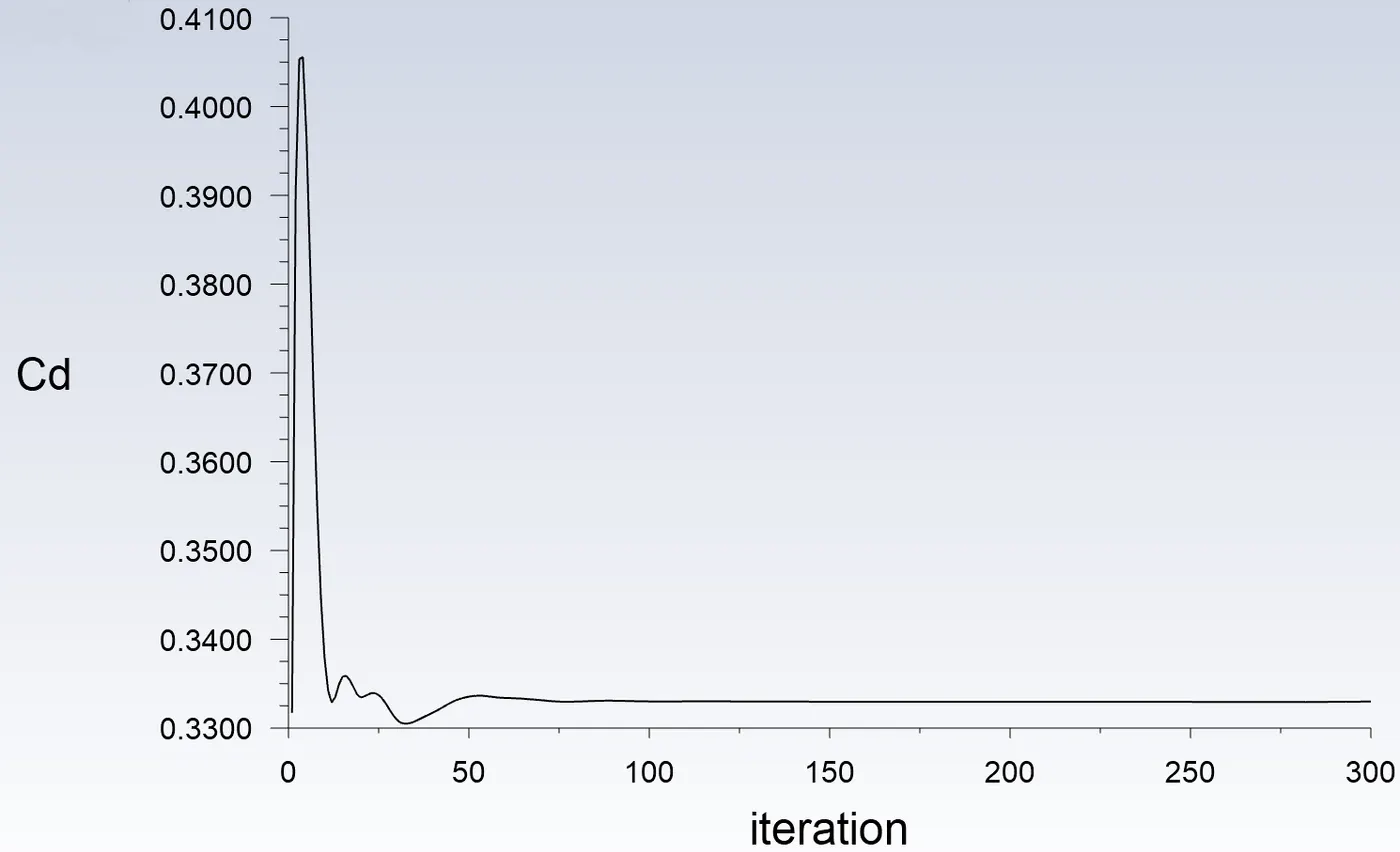
      Residuals and Solution Plot -

          

          

          

          

          

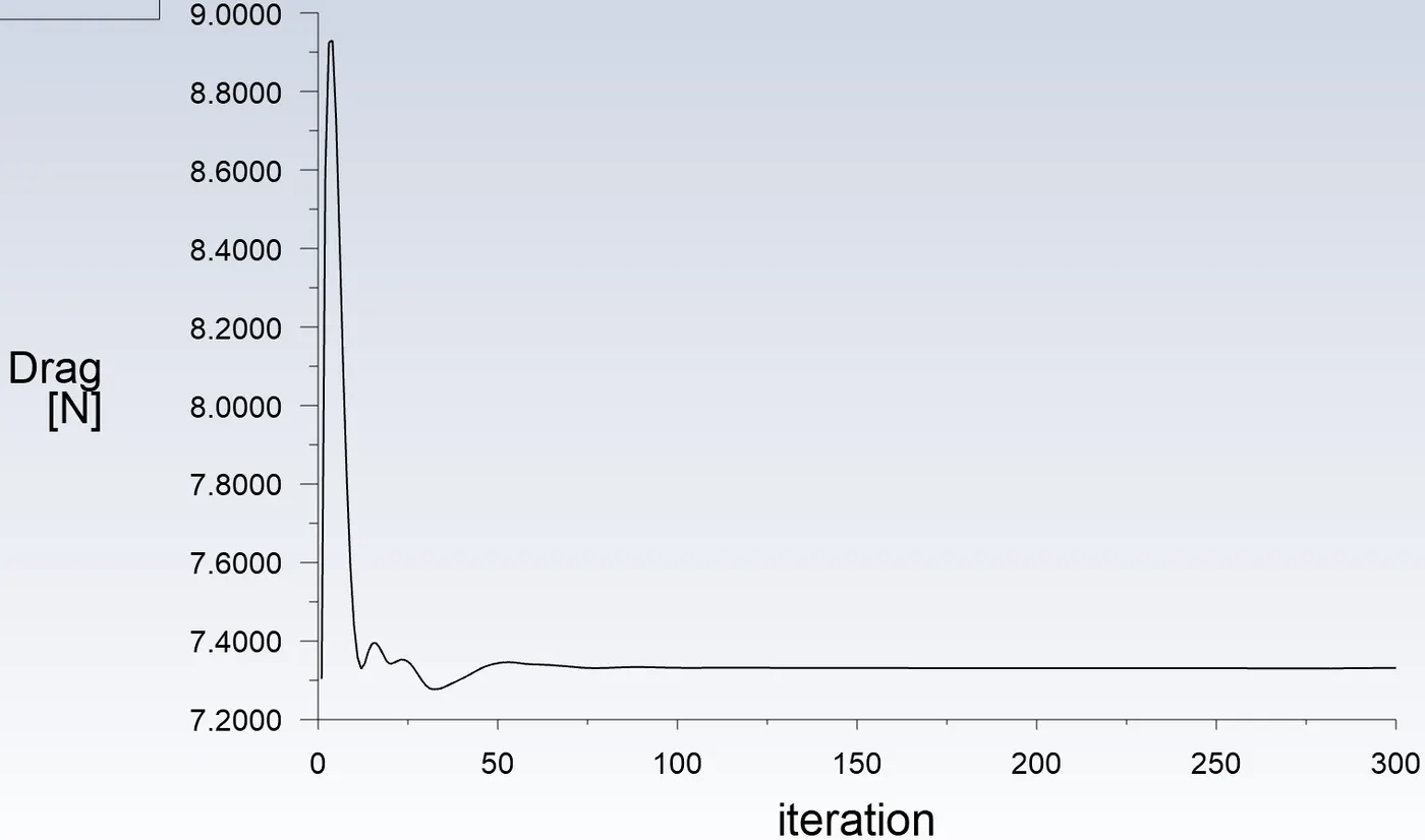
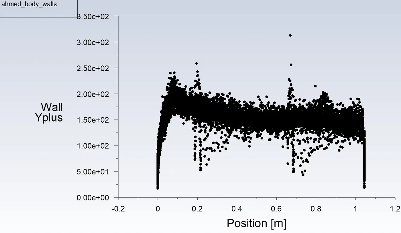
     Contour Plots -

          Velocity Contour -

          

          

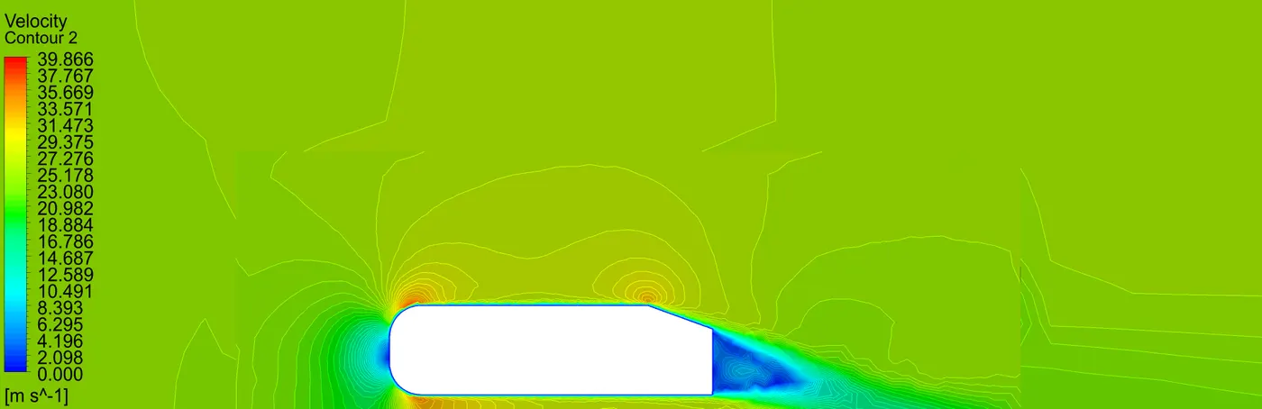
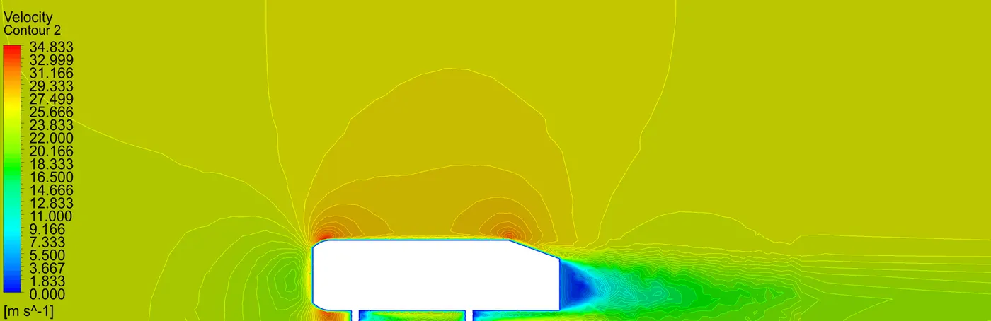
          Pressure Contour - 

          

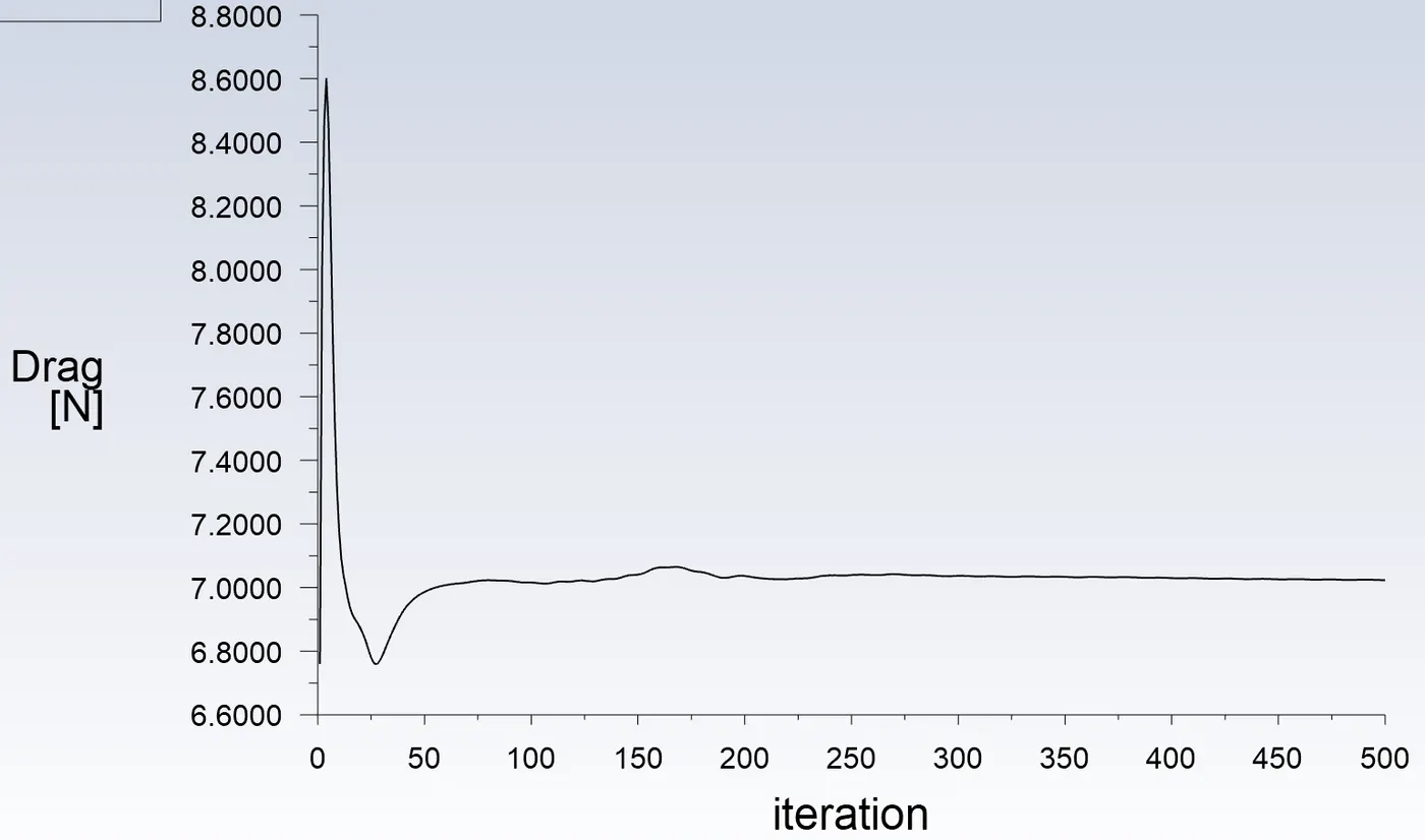
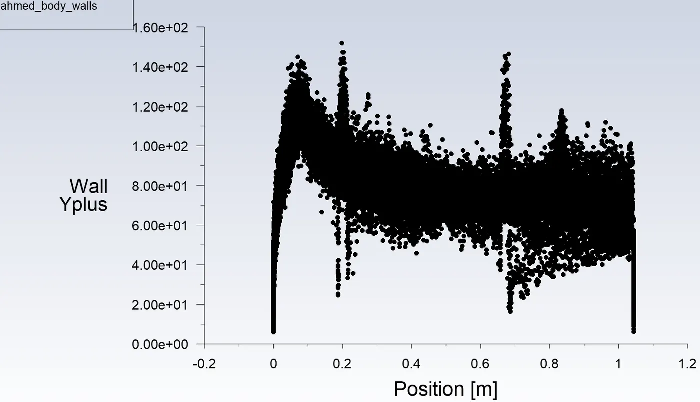
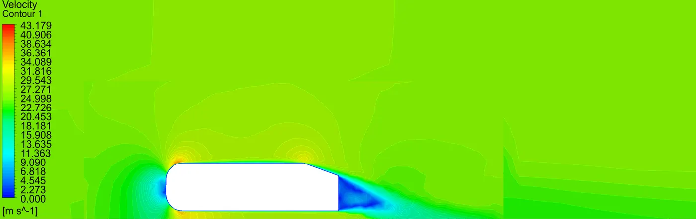
3. For Mesh Config. 2 with k-Omega SST -

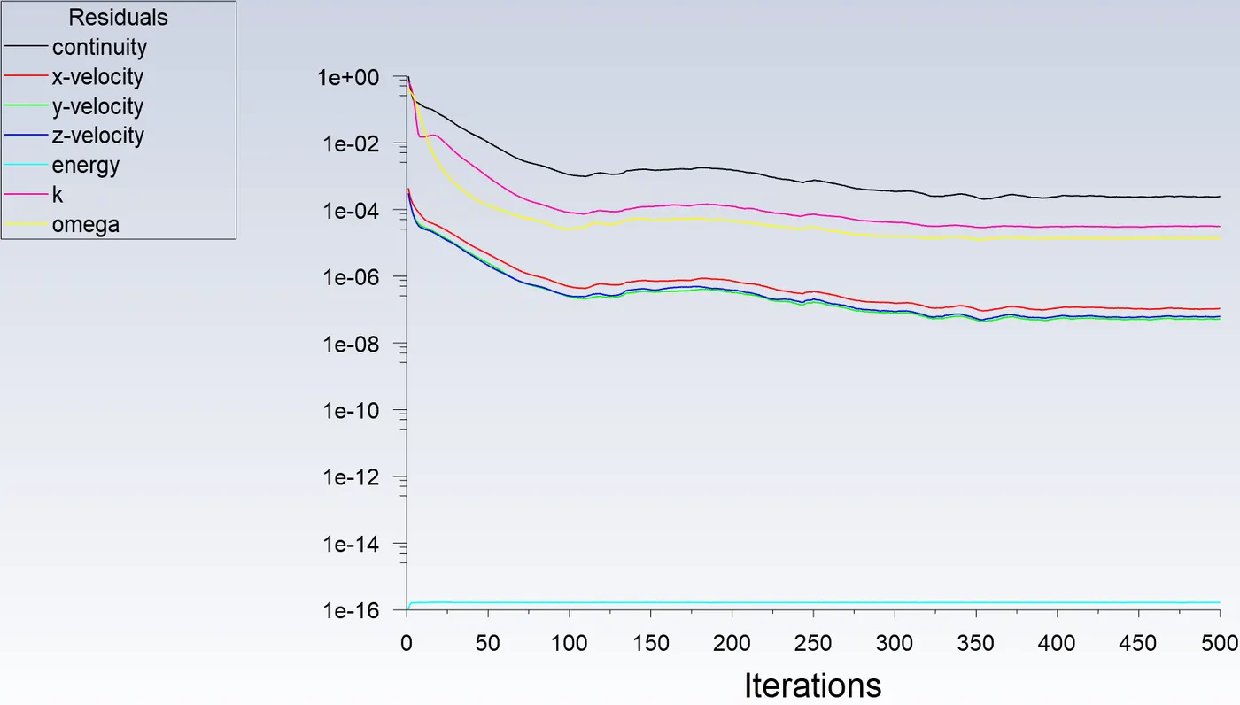
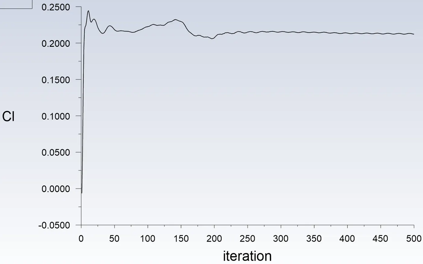
      Residuals and Solution Plot -

          

          

          

          

          

     Contour Plots -

          Velocity Contour -

          

          

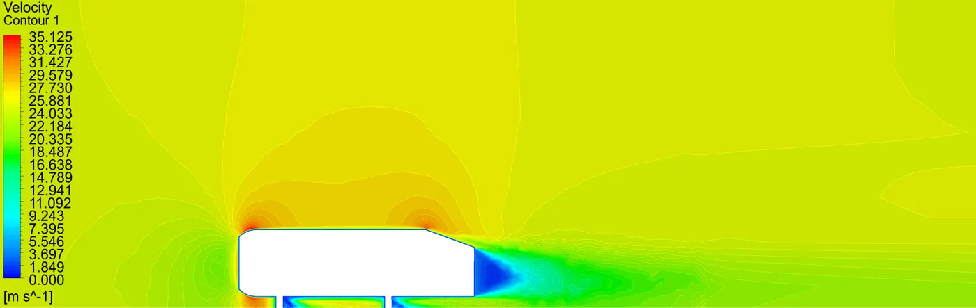
          Pressure Contour - 

          

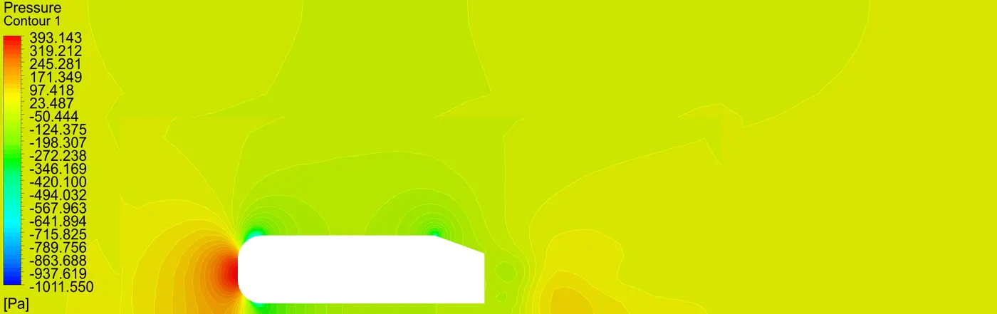
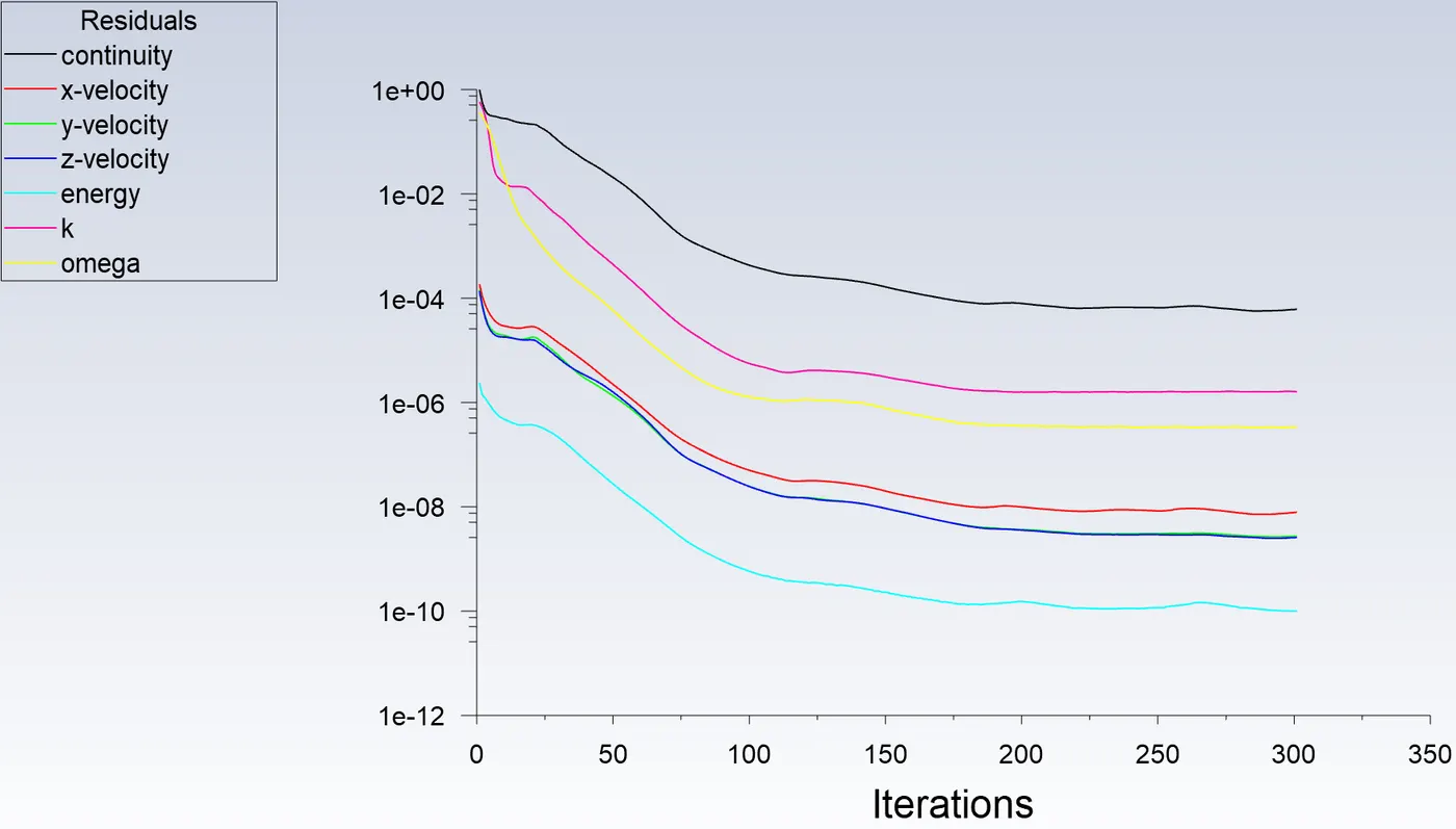
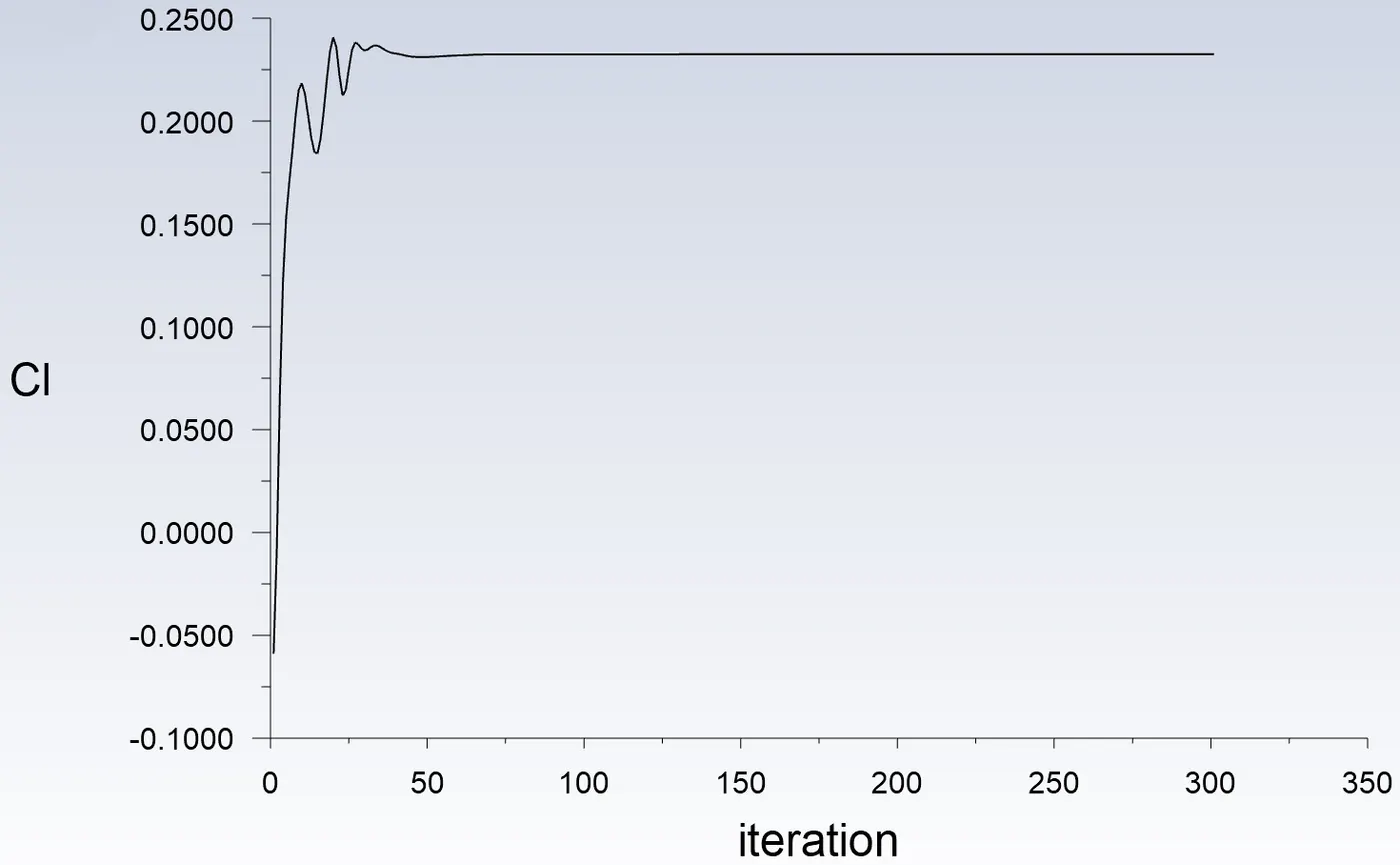
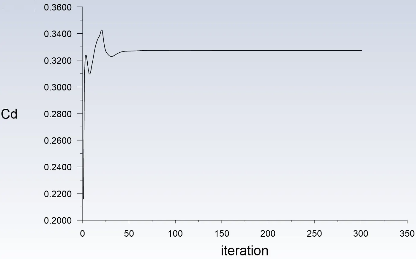
4. For Mesh Config. 3 with k-Omega SST -

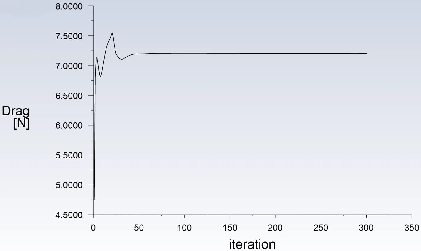
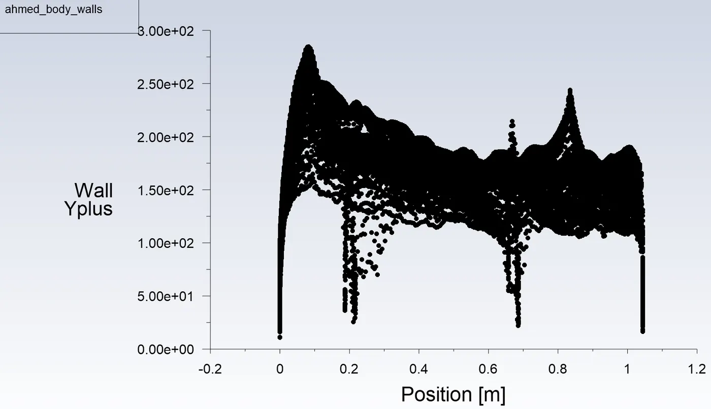
      Residuals and Solution Plot -

          

          

          

          

          

     Contour Plots -

          Velocity Contour -

          

          

          Pressure Contour - 

            

          

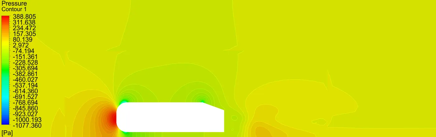
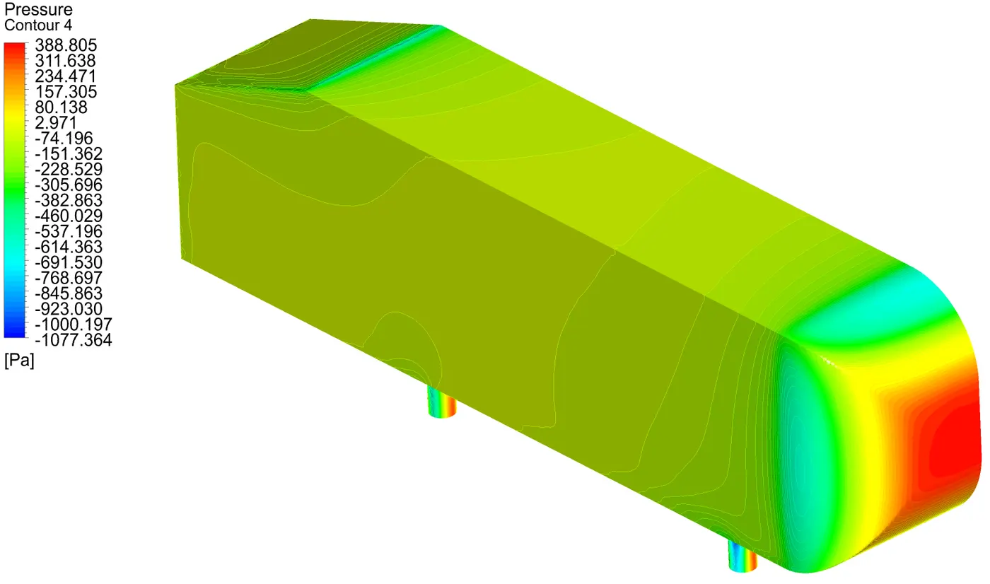
           Vector Plot -

           

           Streamline Plot -

                    

          

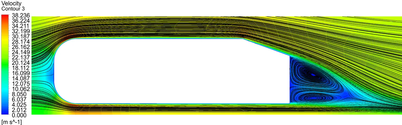
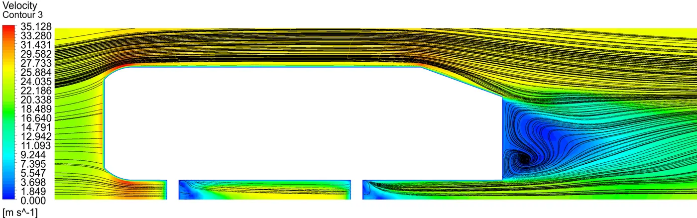
          Wake Streamline -

           

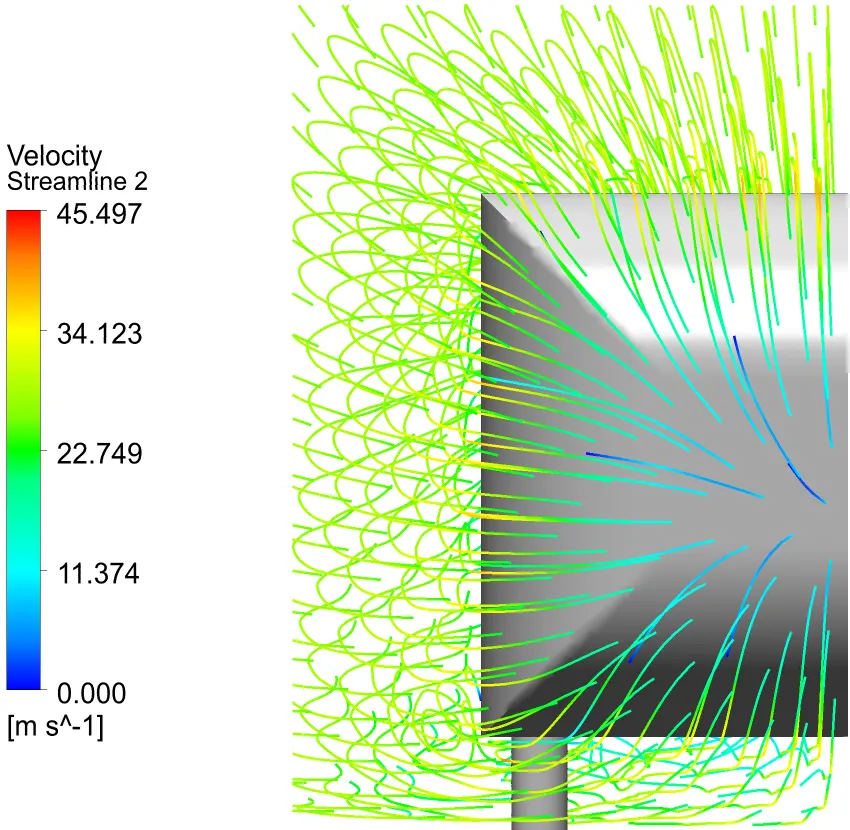
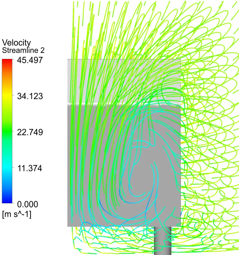
           Animations -

           <iframe src="//www.youtube.com/embed/SrPl_Bwob4U" allowfullscreen="allowfullscreen"></iframe>

           <iframe src="//www.youtube.com/embed/eHbKuikvUcY" allowfullscreen="allowfullscreen"></iframe>

           <iframe src="//www.youtube.com/embed/Akgiz2tr5qM" allowfullscreen="allowfullscreen"></iframe>

RESULTS : 

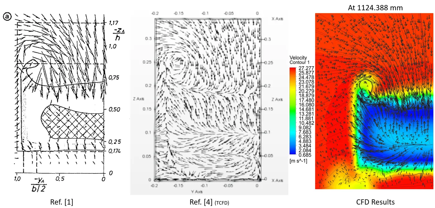
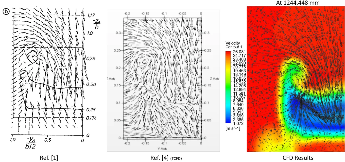
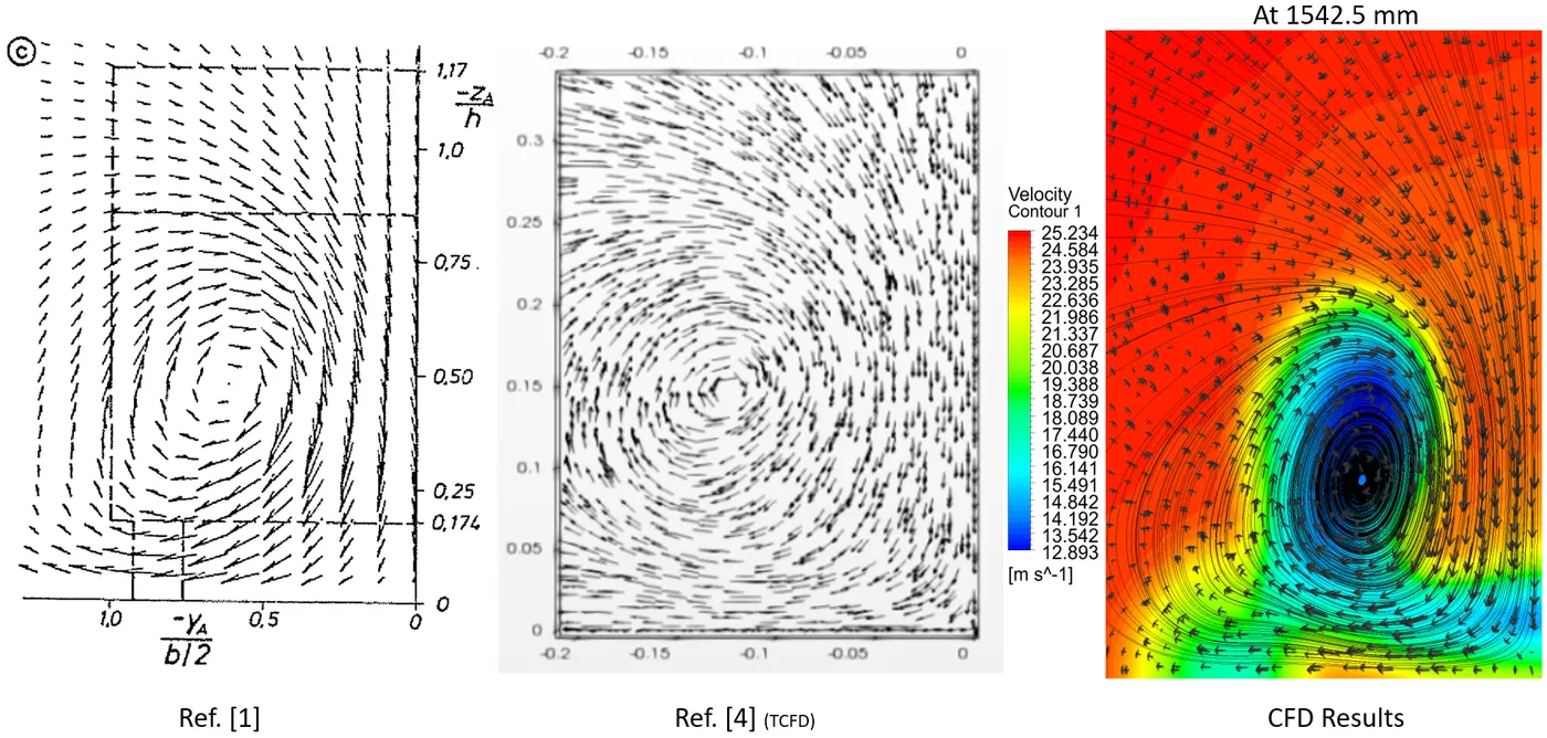
       Experimental Results, Ref.[1] -

      

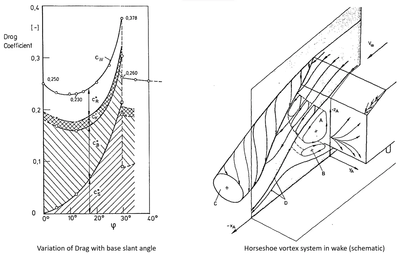
      Following is comparison of the wake at the different position -

                                                

1)  

      

2)

      

3)

      

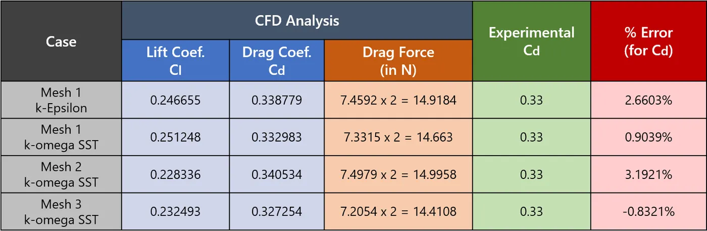
      The Following are the summary report of results of the simulation, -

       

CONCLUSION :

We have successfully performed the analysis of flow over ahmed body.

The appropriate Edge Sizing and Inflation were used for optimum Meshing.

The solver was set up using suitable settings to incorporate the physical phenomena.

We were able to generate required contours for speed, & pressure and visualize streamlines and wake.

The following conclusions can be drawn based on the simulation results after running -

   - We can see all the residuals are less than 10e-3 for every iteration.

   - We have seen that the percentage error for the Drag coefficient is less than five percent in all the case. 

   - We have seen a rise in percentage error from Mesh Configuration 1 to Mesh configuration 2. This may be because Mesh1 does not have inflation layer on the body walls while the Mesh 2 has and therefore there may be lower element quality in the near walls due inflation wall like Orthogonal quality and Aspect ratio.

   - Finally on the Mesh config. 3 we can see the Percentage error of Cd is the lowest, and have more Resolution for the wake region due the more refined mesh.

For further, we can run simulation by creating an structured meshing. 

REFERENCE :

1. S.R. Ahmed, G. Ramm, and G. Faltin, “Some Salient Features of the Time-Averaged Ground Vehicle Wake,” SAE Technical Paper 840300, 1984.
2. H. Lienhart and S. Becker, “Flow and Turbulence Structure in the Wake of a Simplified Car Model,” Lehrstuhl für Strömungsmechanik (LSTM) Universität Erlangen-NürnbergCauerstr. 4, 91058 Erlangen, Germany
3. Hinterberger, C., M. García-Villalba, W. Rodi (2004) Large eddy simulation of flow around the Ahmed body. In: McCallen R, Browand F, Ross J (Eds.) Lecture notes in applied and computational mechanics / The aerodynamics of heavy vehicles: trucks, busses, and trains,Springer Verlag.
4. https://www.cfdsupport.com/ahmed-body-tcfd-benchmark.html
5. Airflow over an Ahmed Body, COMSOL; https://www.comsol.com/model/airflow-over-an-ahmed-body-8565