Week 4 - CHT Analysis on Exhaust port

AIM : To perform Conjugate Heat Transfer Analysis of Exhaust port.

OBJECTIVES :

• Setting up the Geometry in Spaceclaim.
• Create optimal meshing for the model in Ansys Mesher.
• Get Results for inlet velocity of 5m/sec and temperature 700K.
• Setup the model for the analysis from the given data,select a proper turbulence model and maintain the correct Y plus value.
• Run the simulation and Post Process the results.
• Validate the result and Verify if the Heat transfer coef. predictions from the simulations are right or not.
• State on what factors does the accuracy of the prediction depend on

INTRODUCTION :

Conjugate Heat Transfer (CHT) is a significant concept in the field of thermal engineering, playing a crucial role in various industrial and technological applications. It involves the study of heat transfer in a system where multiple modes of heat transfer like conduction, convection, and radiation occur simultaneously. These modes interact with each other, making the heat transfer process complex and challenging to analyze.

Conjugate Heat Transfer and its simulations are indispensable tools in thermal engineering, providing valuable insights into complex heat transfer processes and aiding in the design and optimization of various thermal systems. The simulations are performed using Computational Fluid Dynamics (CFD) software that solves the governing equations of fluid flow and heat transfer. The accuracy of these simulations depends on the correct representation of boundary conditions, material properties, and the numerical methods used for solving the equations.

Turbulence Model

The K-Omega SST and K-Epsilon are two popular turbulence models used in Computational Fluid Dynamics (CFD), each with its unique strengths.

The K-Omega SST (Shear Stress Transport) model is a blend of the K-Omega and K-Epsilon models, designed to leverage the advantages of both. It uses the K-Omega formulation in the near-wall region, making it directly usable through the viscous sub-layer, thus eliminating the need for damping functions. This leads to better accuracy and robustness in complex boundary layer flows under adverse pressure gradients and separations. Furthermore, it switches to a K-Epsilon behavior in the free-stream, thereby reducing sensitivity to the inlet free-stream turbulence properties.

On the other hand, the K-Epsilon model is a general-purpose model that assumes isotropic turbulent viscosity. It is widely used for a range of applications, particularly those involving high Reynolds number flows with relatively small pressure gradients. However, it may not be as accurate as the K-Omega SST model in near-wall regions or for flows with significant pressure gradients.

In conclusion, while both models are powerful tools for solving turbulence problems in CFD, the choice between them depends on the specific requirements of the flow problem at hand. The K-Omega SST model is generally preferred for more complex flows with adverse pressure gradients and separations, while the K-Epsilon model is often used for simpler, high Reynolds number flows.

Near-Wall Treatment in Computational Fluid Dynamics (CFD) is crucial for accurately capturing the physics of wall-bounded turbulent flows. It involves resolving the viscous sublayer, a region near the wall where viscous effects dominate. This region is characterized by significant gradients in velocity and temperature, making it computationally challenging. Various strategies, such as wall functions and low-Reynolds number models, are employed to handle this. Wall functions provide a bridge between the wall and the fully turbulent region, while low-Re models resolve the entire boundary layer. The choice of strategy depends on the flow problem and computational resources available.

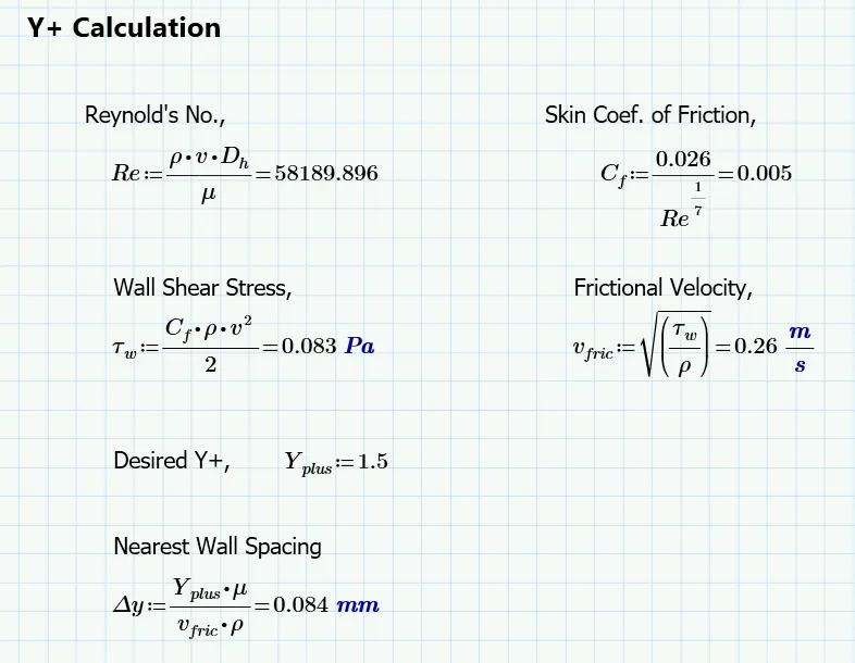
In CFD, Y+ is a non-dimensional wall distance used for near-wall treatment in turbulence modeling. It represents the ratio of inertial forces to viscous forces and varies across the boundary layer. A low Y+ value (<1>30) suggests dominance of inertial forces, allowing use of wall functions to approximate near-wall behavior. Proper Y+ estimation is crucial for accurate simulation results, especially in wall-bounded turbulent flows.

STEPS / PROCEDURE :

1) Geometry

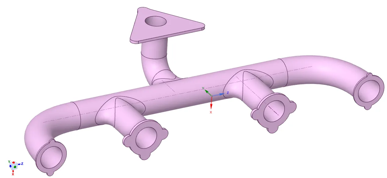
The Following is the geometry based on given Step file & dimensions in spaceclaim -

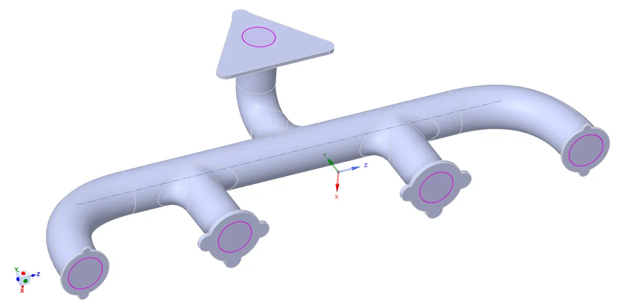
Creating Fluid region using volume extract and then enabling share topology

2) Meshing

After doing Geometry preparation, we gone open the geometry in Ansys Mesher via workbench -

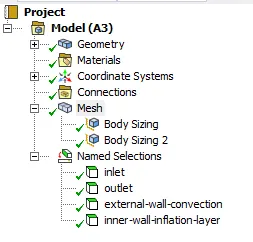
• Creating Named Selections
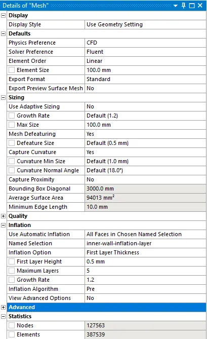
• Assigning proper mesh sizing
• Creating Inflation layers at the surrounding of the wall
• Checkng mesh quality.

Doing Y+ Calculation using S Math Software -

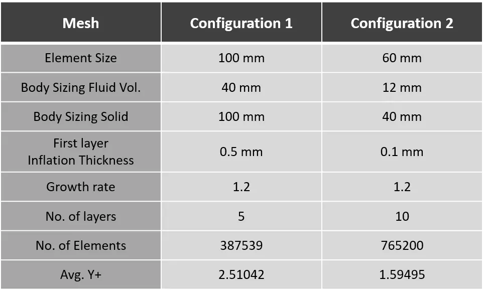
To Check for Mesh Independence We gone do the analysis in following 2 configurations -

Mesh Quality Verification-

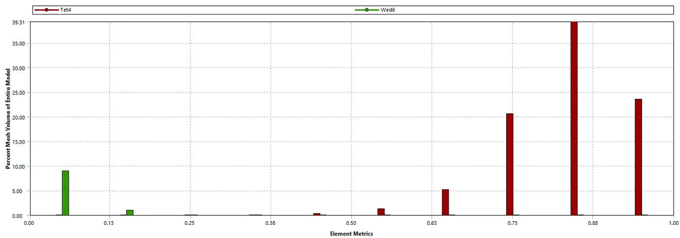
Following is the surface mesh And Element quality of the Case Setup -

i) For Mesh Configuration 1 -

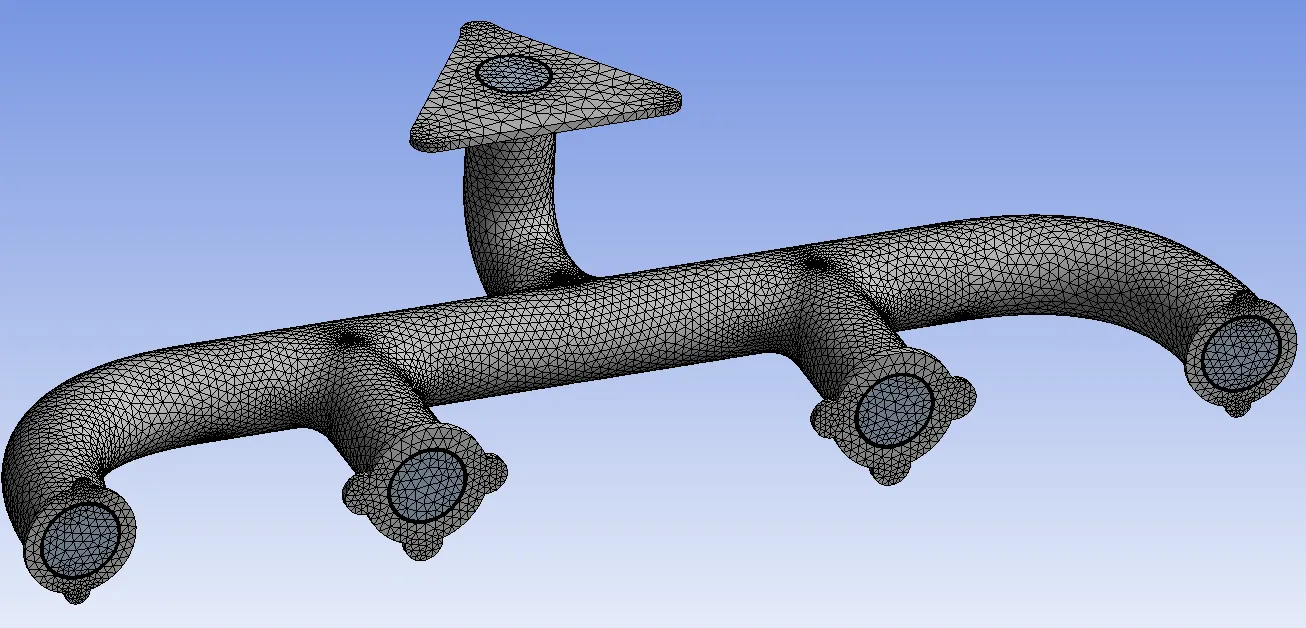
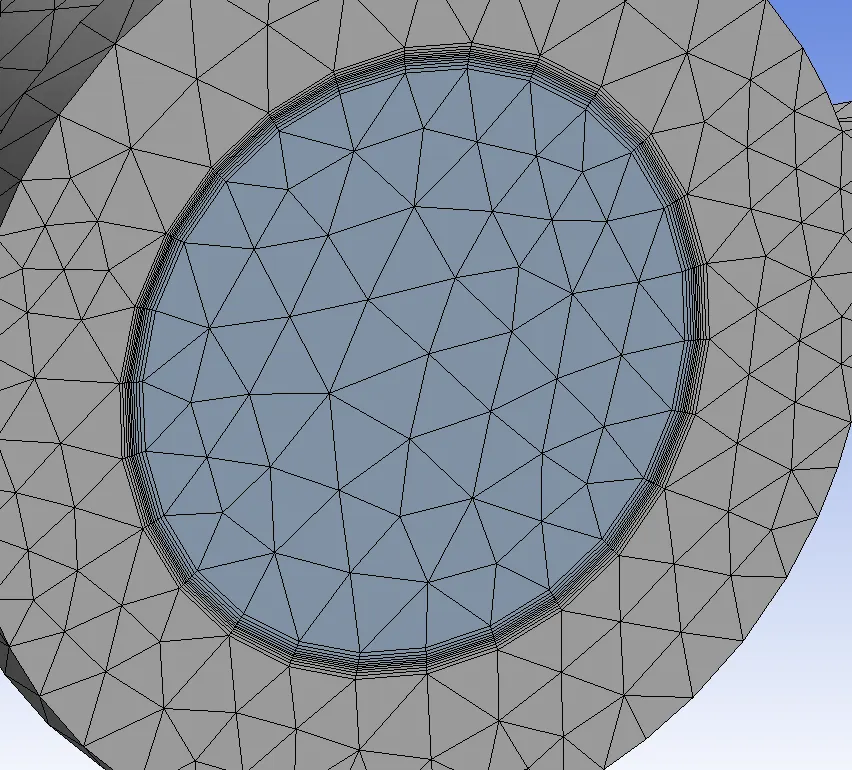
ii) For Mesh Configuration 2 -

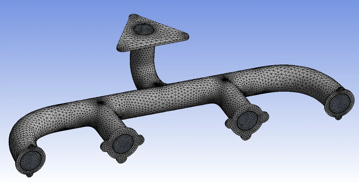
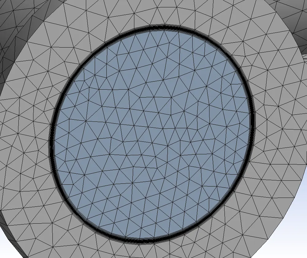
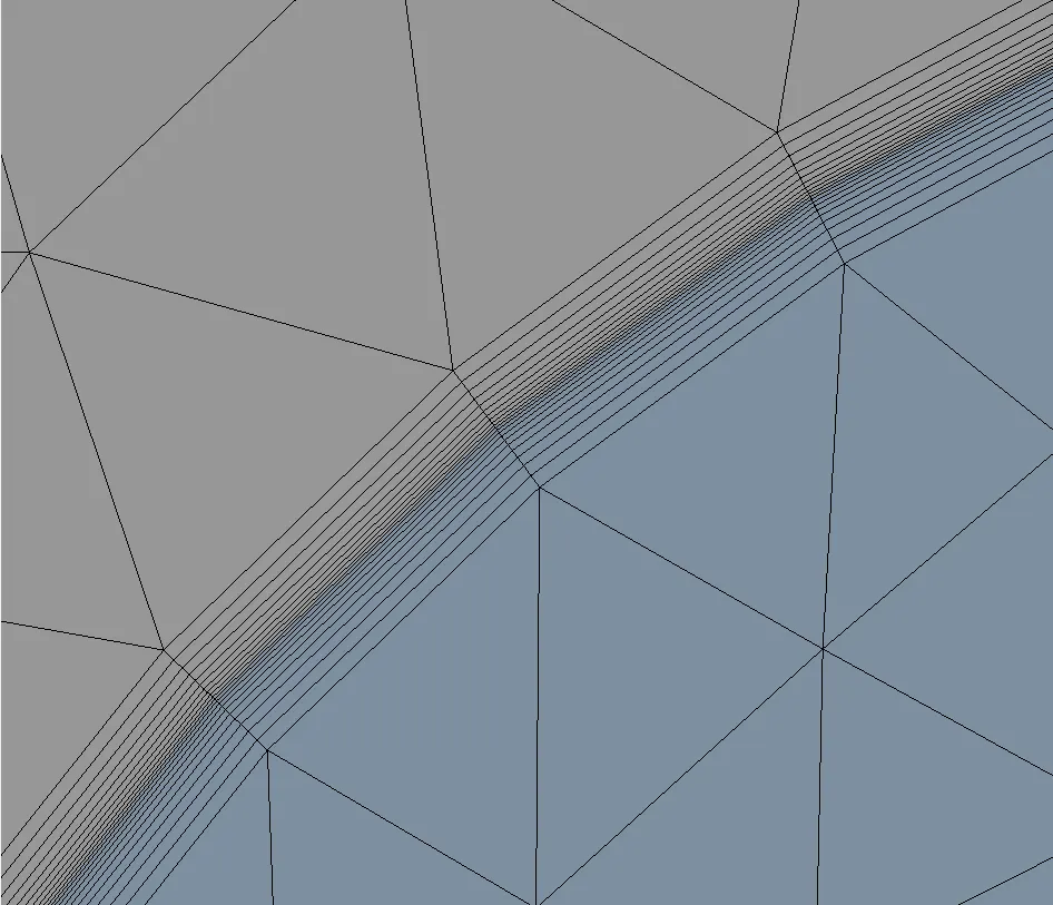
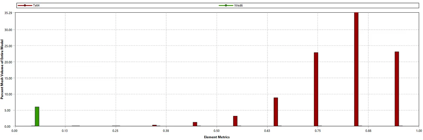
We can the mesh quality is very satisfied. 90% of the mesh cell are lying on good quality range.

3) Solver Settings -

Closing the Mesher & opening the Fluent Solver from the workbench

Checking the the Double precision option and selecting no. of parallel process.

Setting solver settings and initialization values.

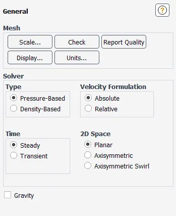
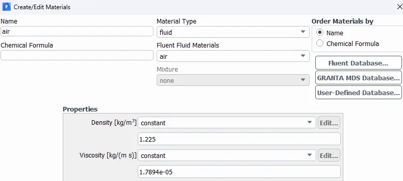
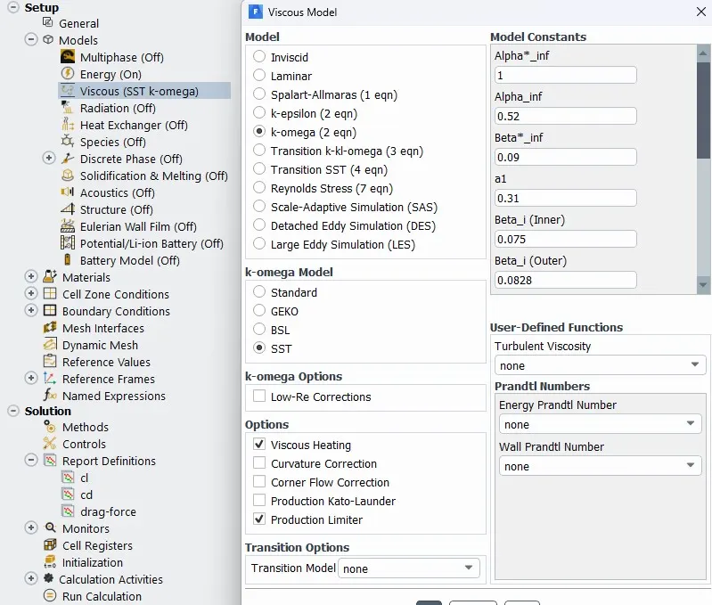
Selecting the turbulence model and its settings.

Setting Inilization, here we are using Hybrid Initialization.

Creating Solution reports.

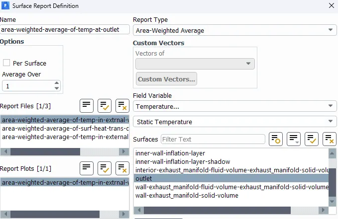
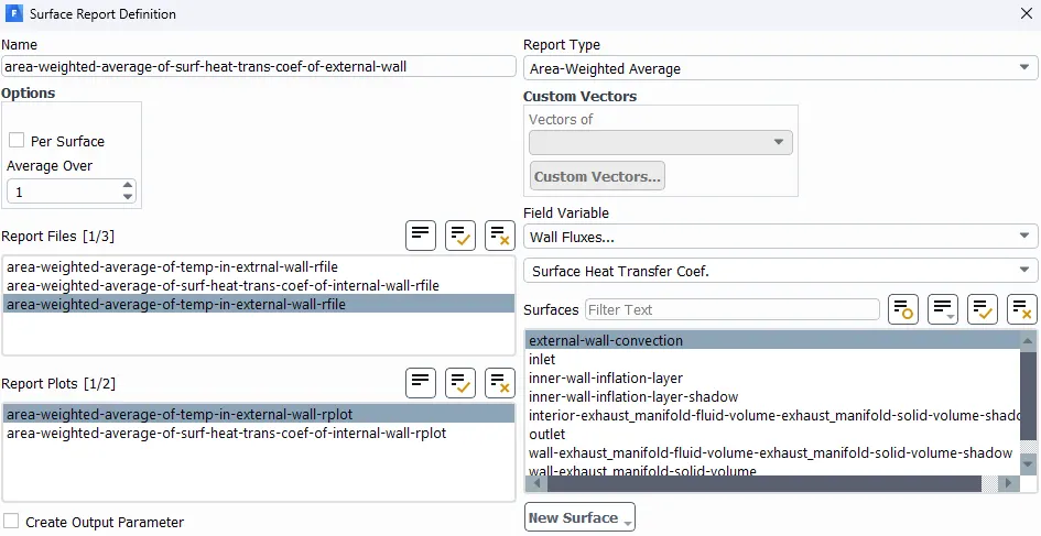
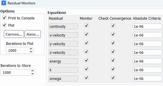
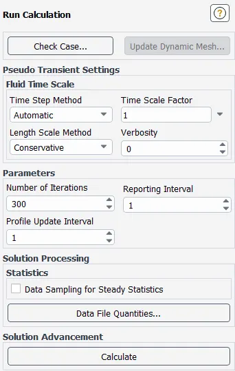
The convergence criteria has been turned off since we have monitor flow with respect to time.

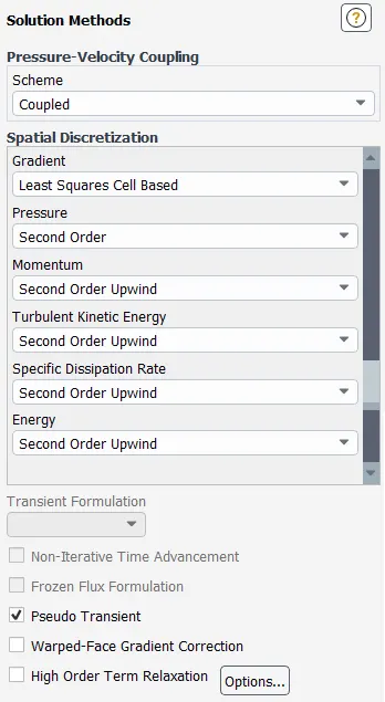
Keeping the Solution method & discretization schemes as shown below.

POST PROCESSING :

Outputs

1. For Mesh Config. 1 -

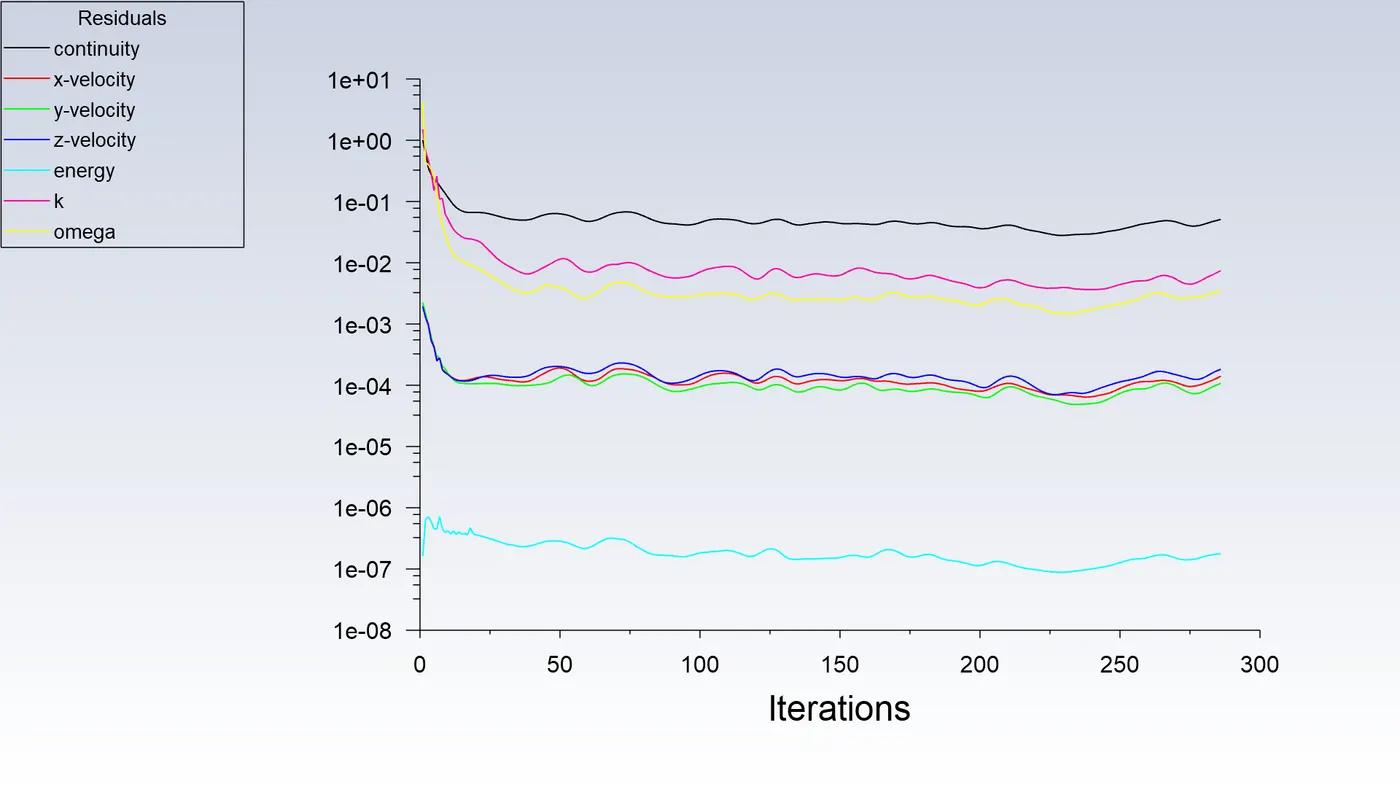
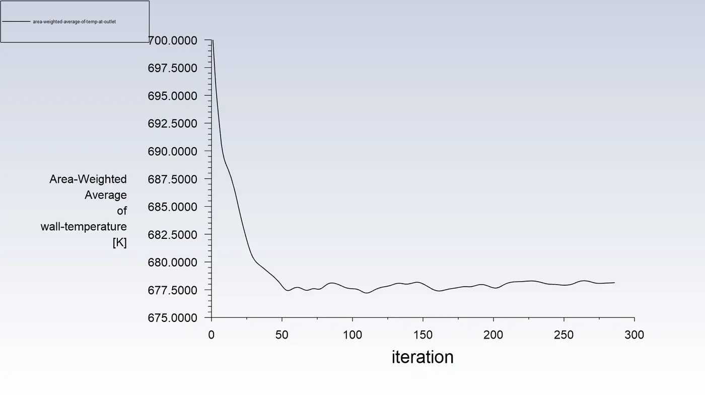
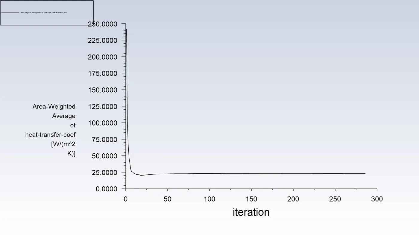
Residuals and Solution Plot -

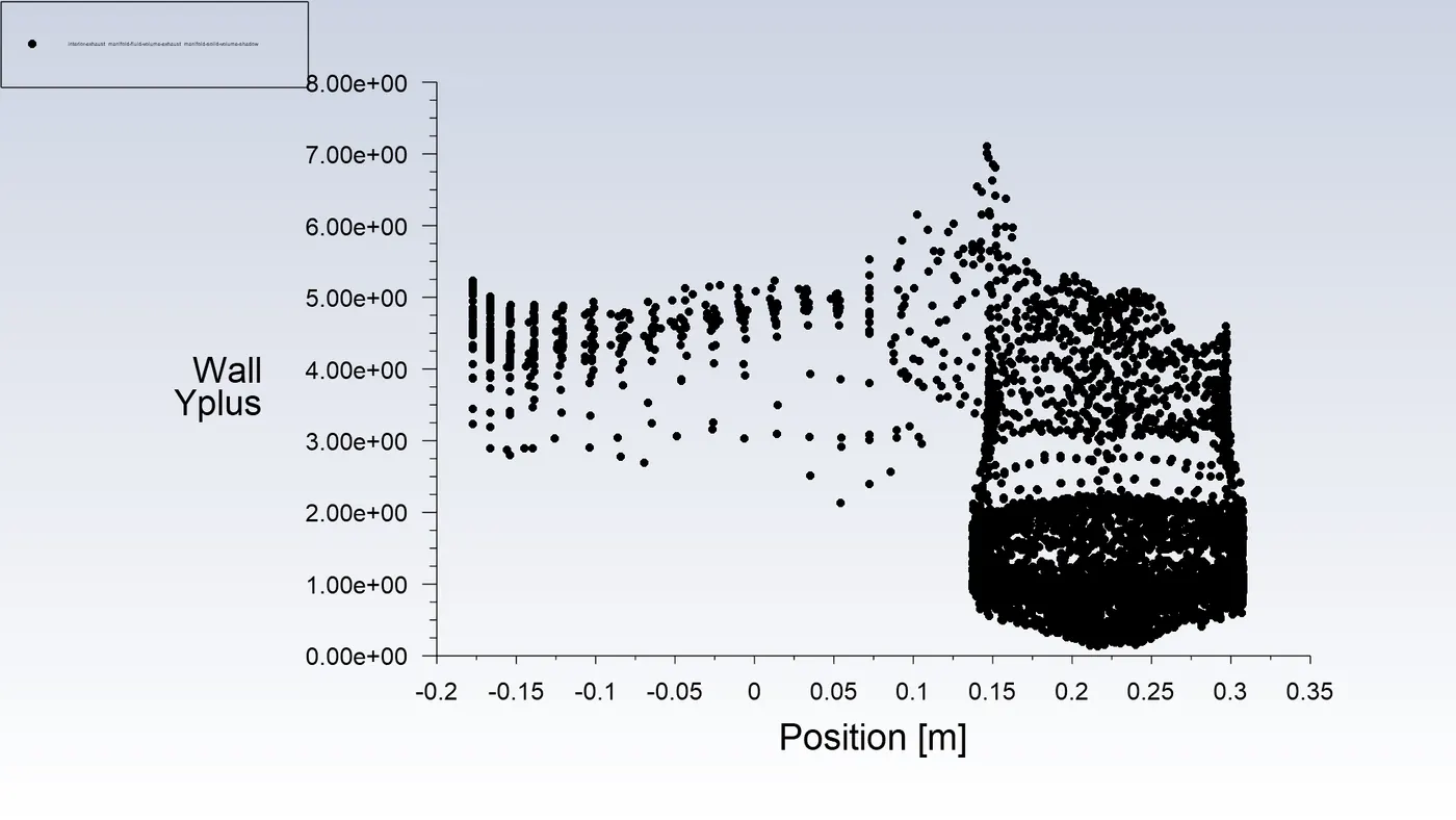
Contour Plots -

Velocity Contour -

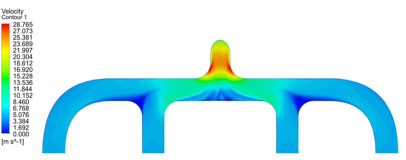
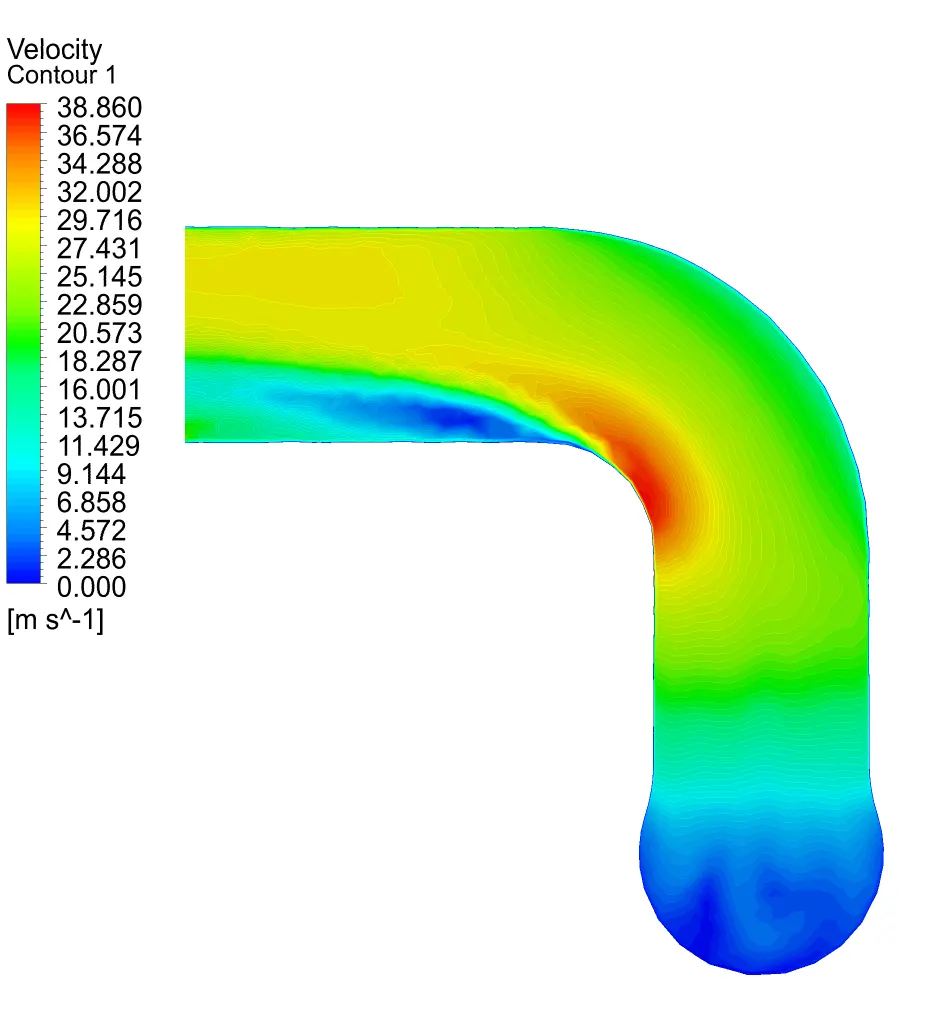
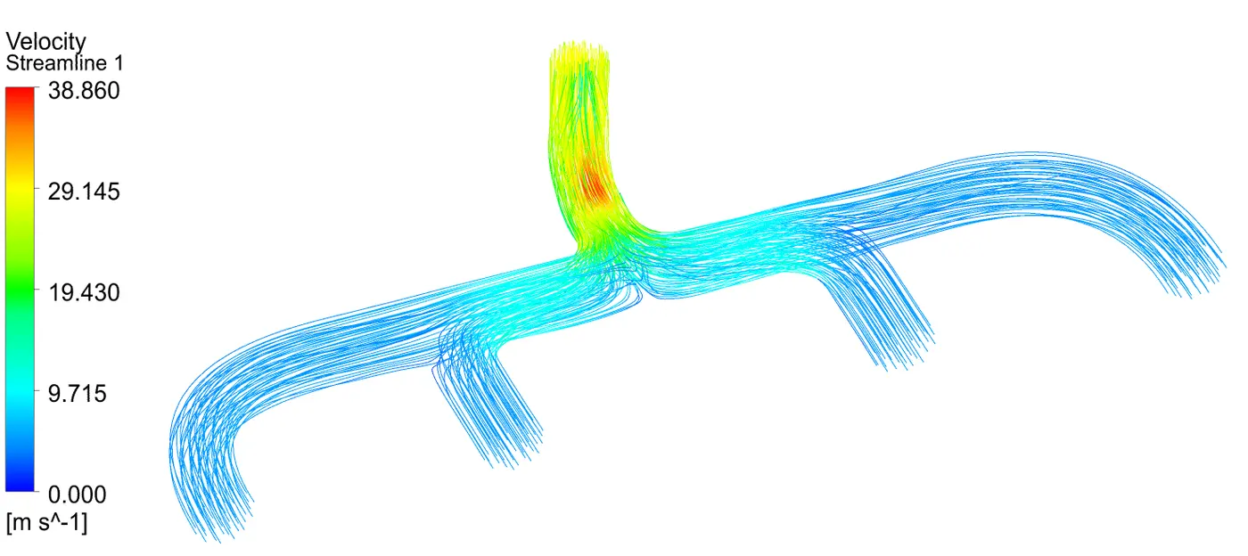
Pressure Contour -

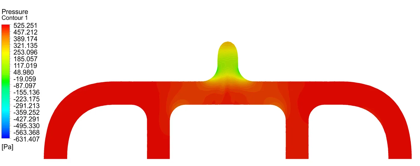
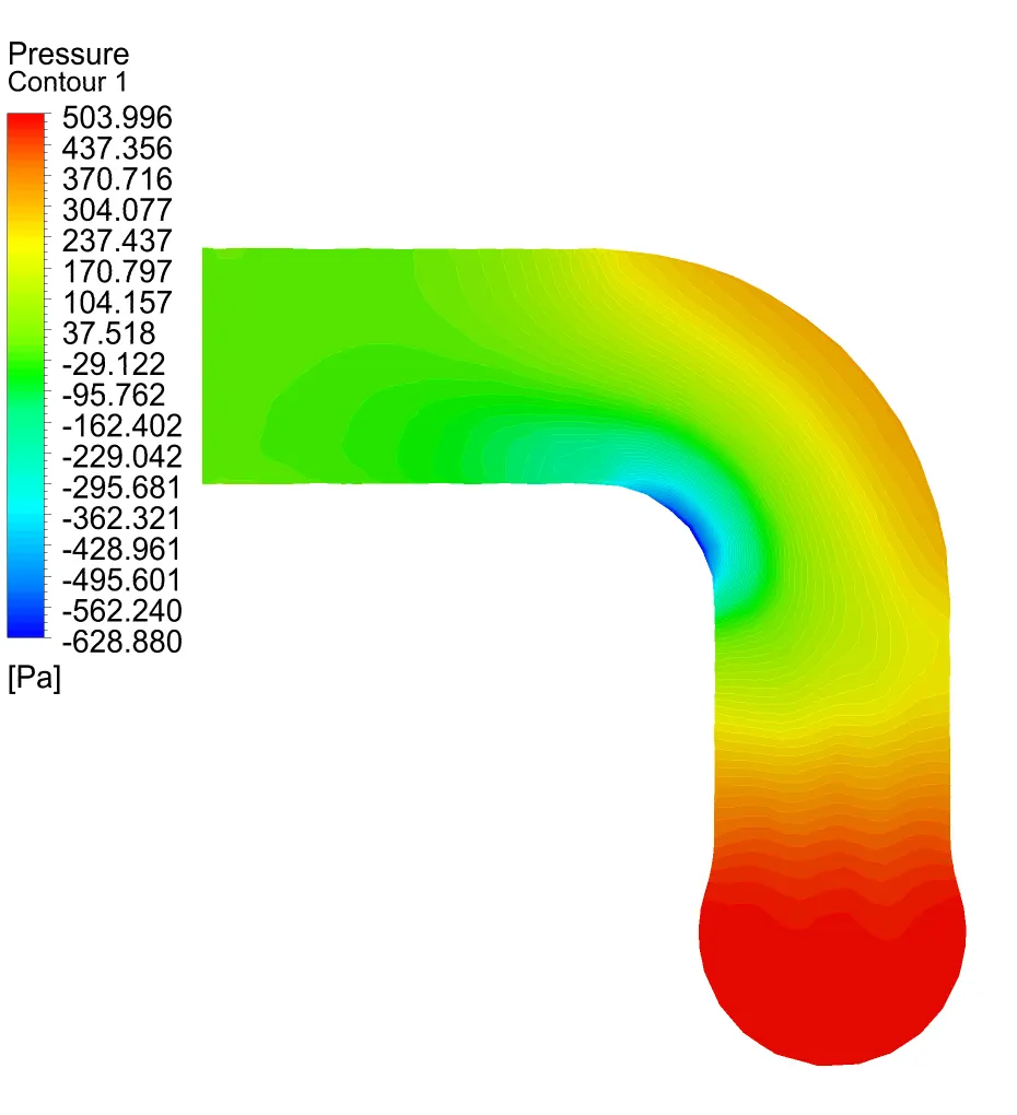
Temperature Contour -

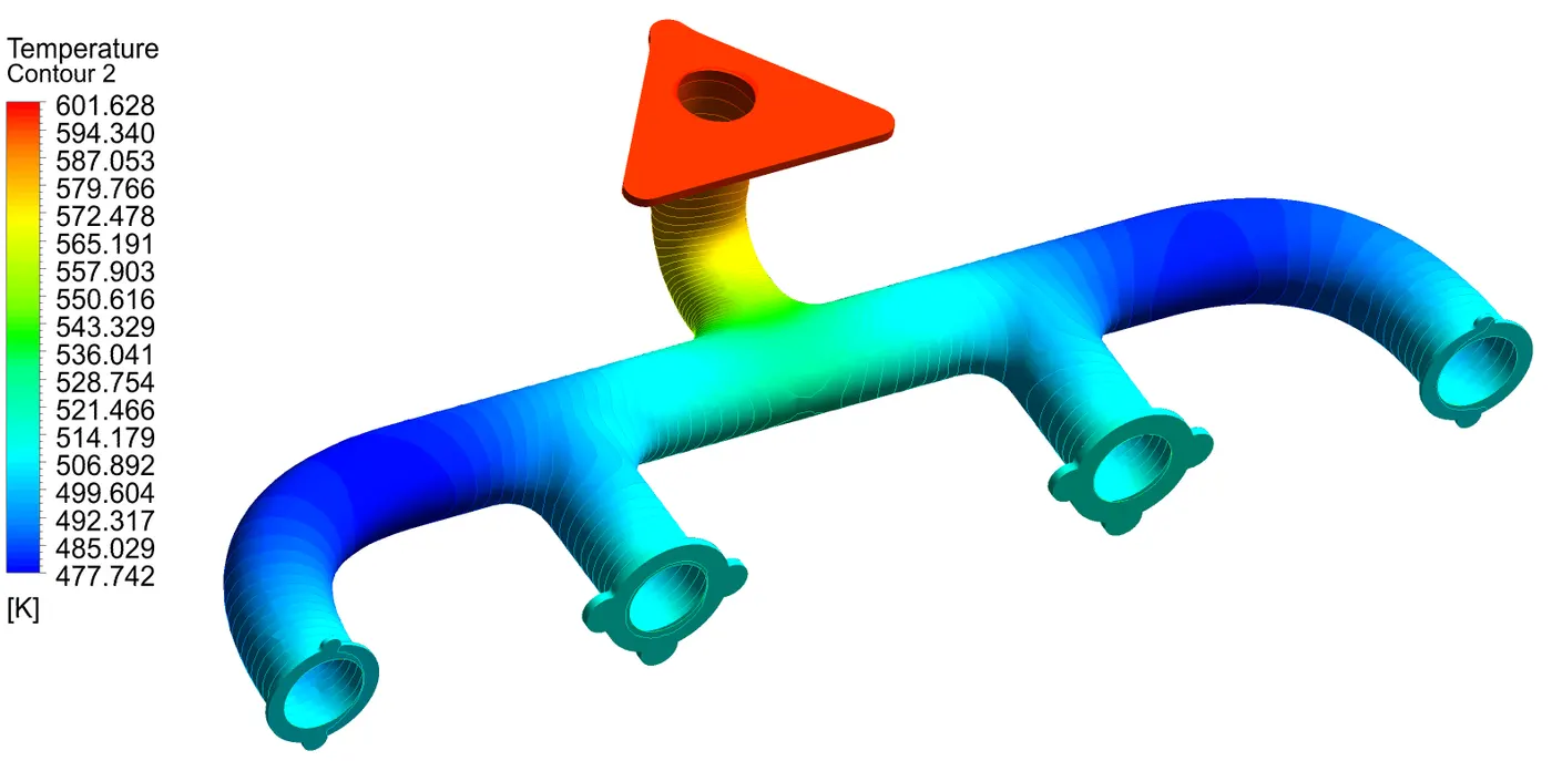
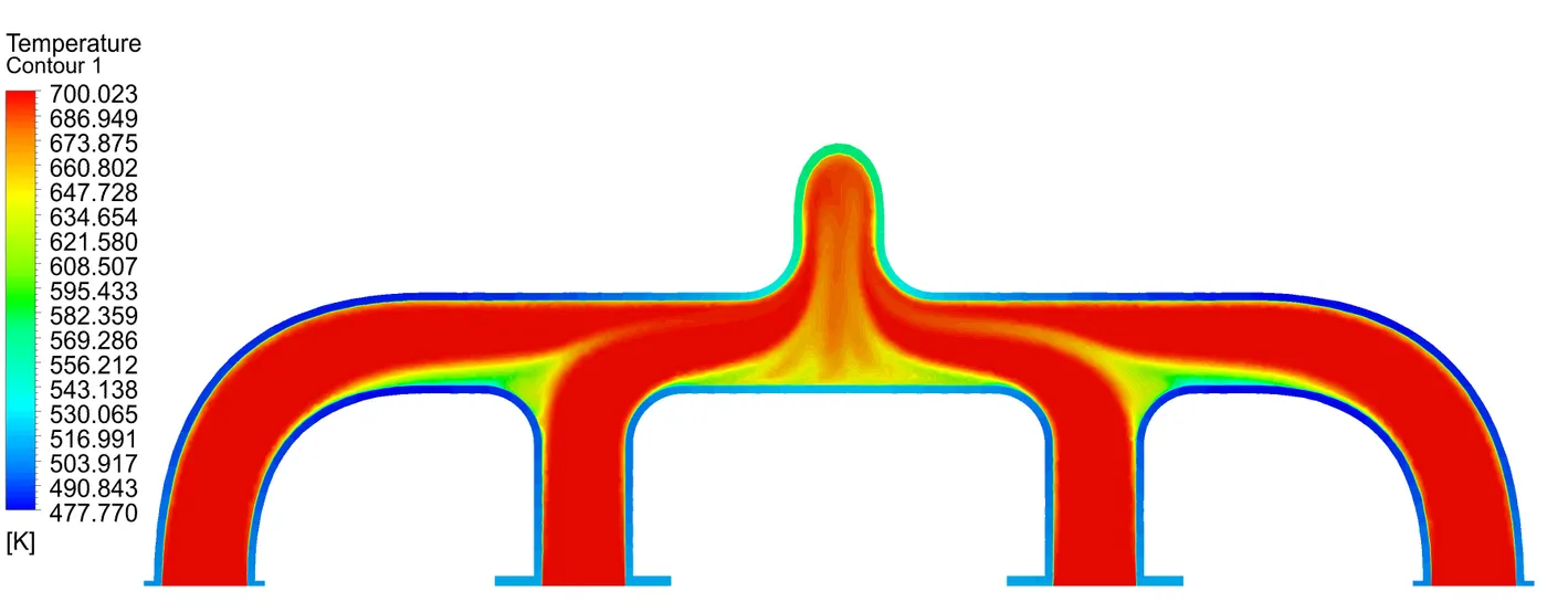
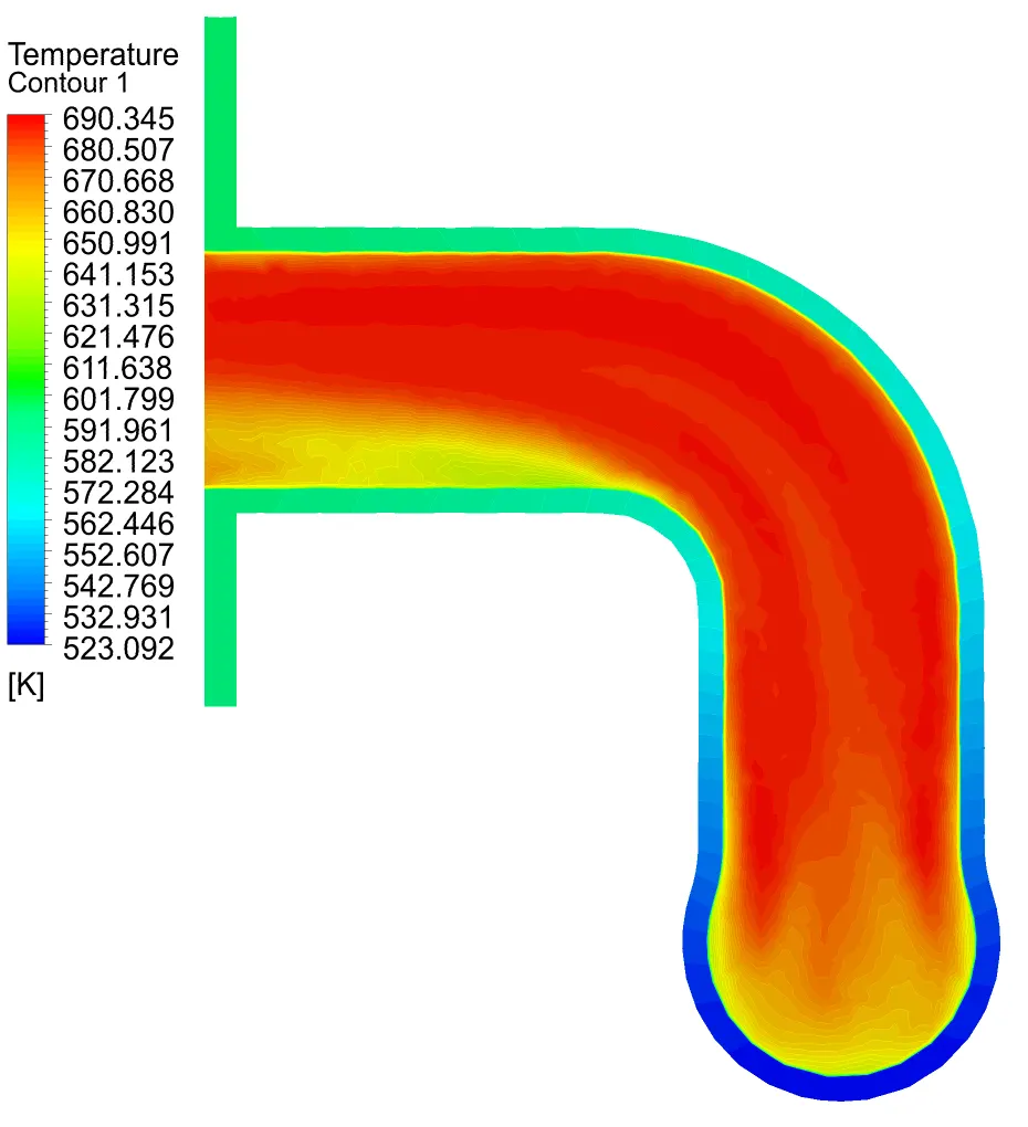
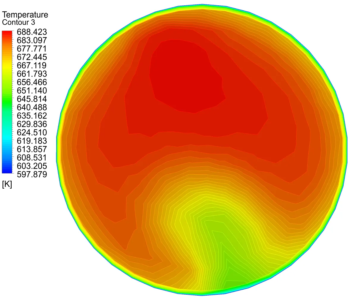
2. For Mesh Config. 2 -

Residuals and Solution Plot -

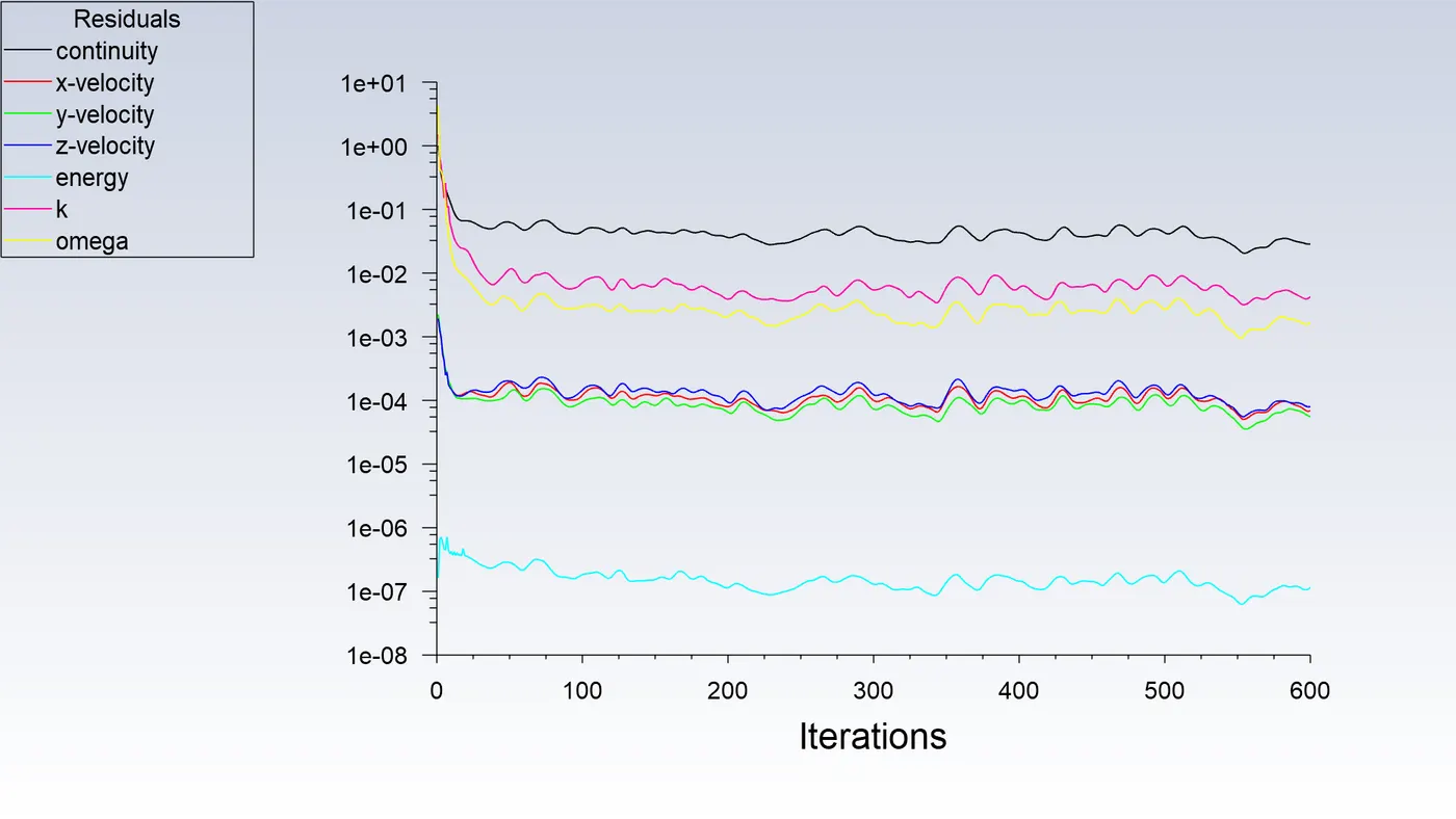
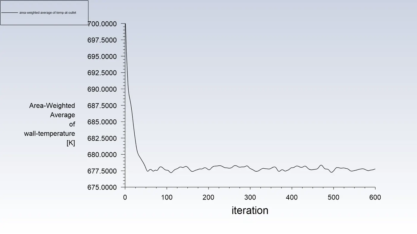
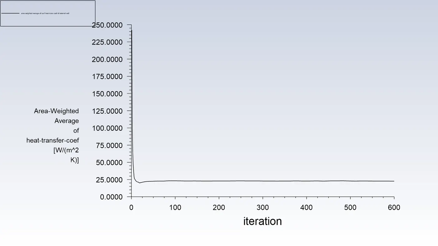
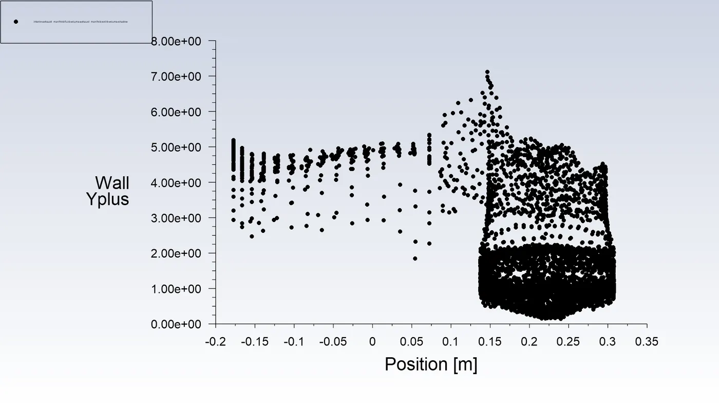
Contour Plots -

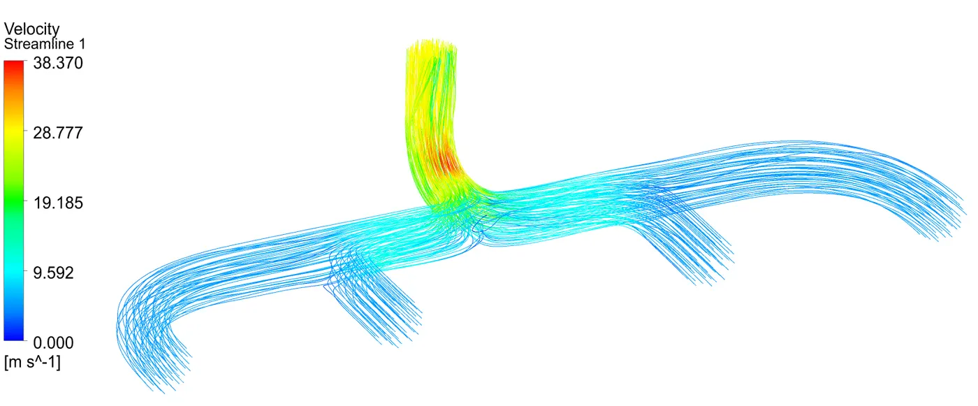
Velocity Contour -

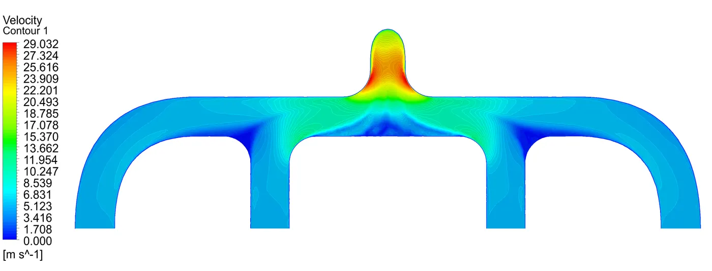
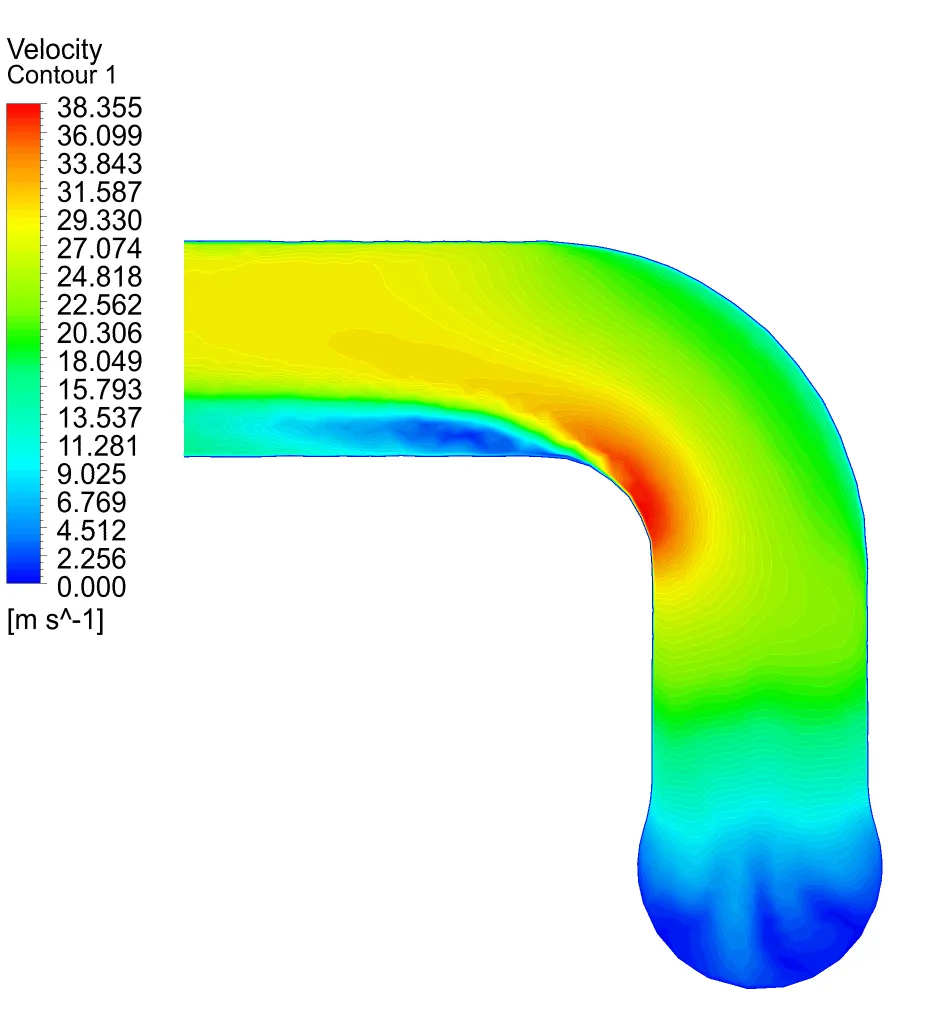
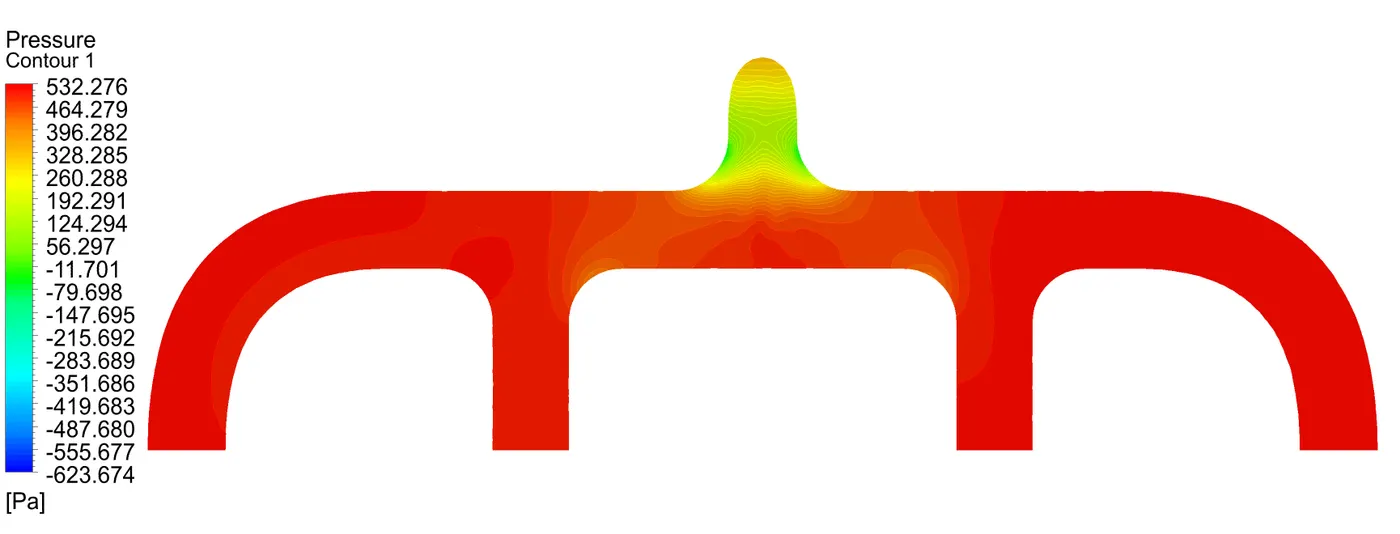
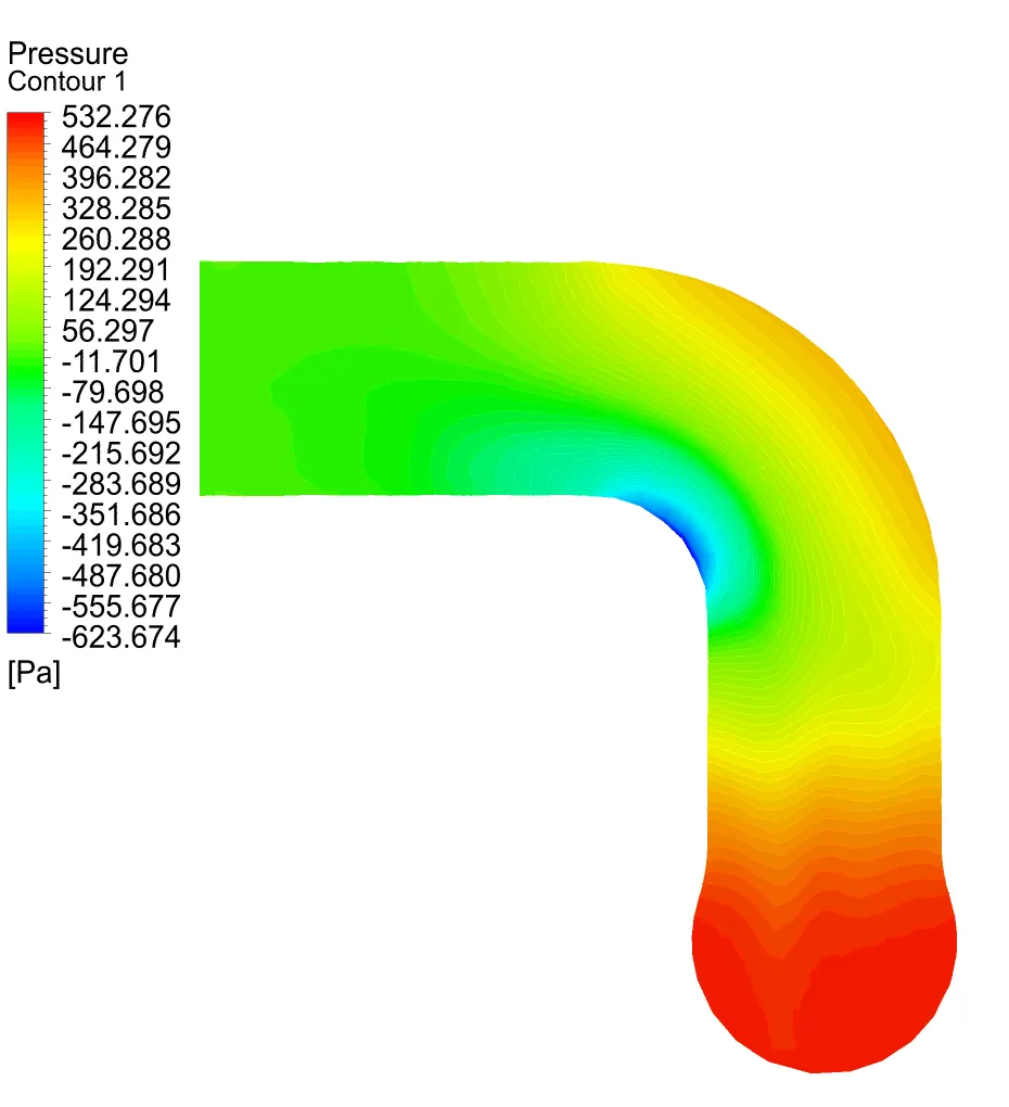
Pressure Contour -

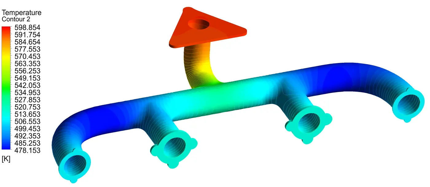
Temperature Contour -

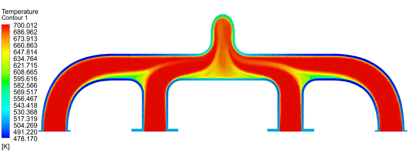
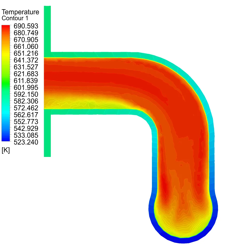
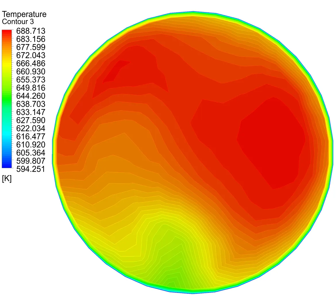
Animation -

VERIFICATION & VALIDATION :

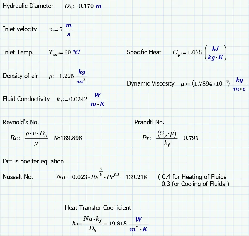
Doing Analytical Calculation for Validation Using S Math Software -

RESULTS :

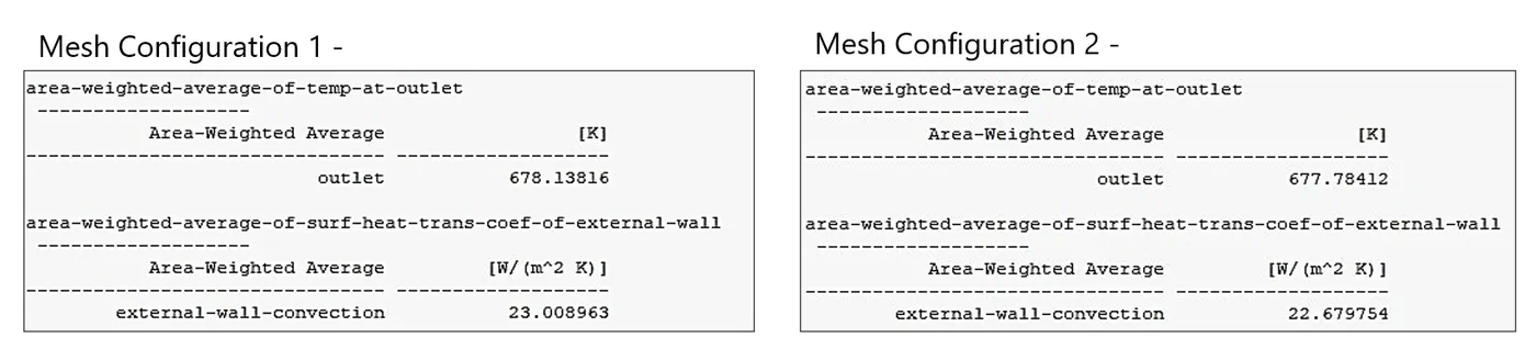
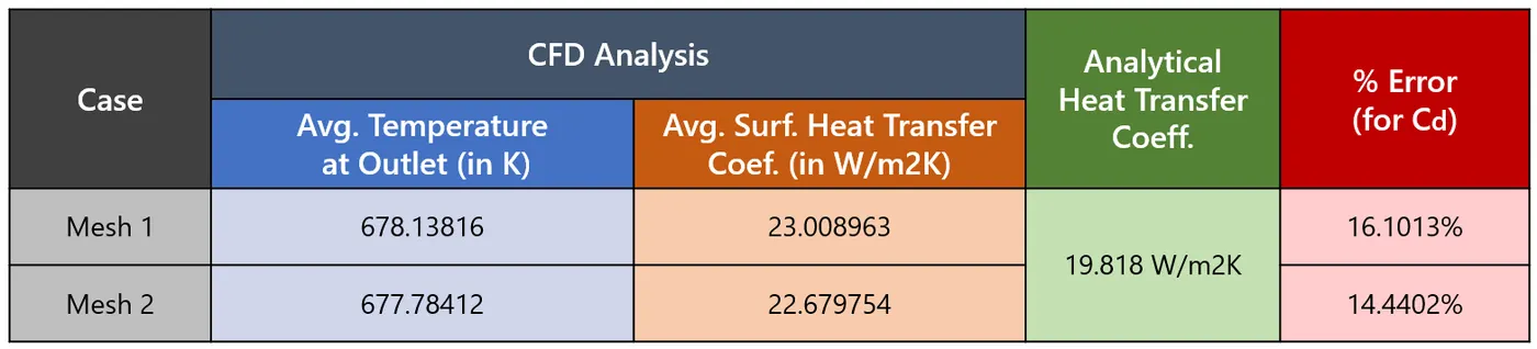
The Following are the summary report of results of the simulation, -

CONCLUSION :

We have successfully performed the CHT analysis of Exhaust Port.

The appropriate Edge Sizing and Inflation were used for optimum Meshing.

The solver was set up using suitable settings to incorporate the physical phenomena.

We were able to generate required contours for speed, & pressure and visualize streamlines and Temperature Contours.

The following conclusions can be drawn based on the simulation results after running -

- We can see all the residuals are less than 10e-3 for every iteration except Continuity.

- We have seen that percentage error for the Heat transfer Coeffiecient with analytical calculation is less than 20% percent in both cases.

- We have seen a slight reduction in percentage error from Mesh1 to Mesh2/

- The remaining percentage error because of there may be lower element quality in the near walls due inflation wall like Orthogonal quality and high Aspect ratio, which can resolved more refiniment near wall.

REFERENCE :

1. Simulation of Conjugate Heat Transfer Between Engine Head and Cooling Medium of Diesel Engine https://www.researchgate.net/publication/283020042_Simulation_of_Conjugate_Heat_Transfer_CHT_Between_Engine_Head_and_Cooling_Medium_of_Diesel_Engine
2. Conjugate Heat Transfer https://www.comsol.com/blogs/conjugate-heat-transfer/
3. Modeling of Boundary Layer and the Influence on Heat transfer with help of CFD - https://aip.scitation.org/doi/pdf/10.1063/1.5081654
4. Measurement of the heat transfer coefficient -https://www.sciencedirect.com/science/article/abs/pii/0360132396000145
5. K-omega and K-omega SST - https://www.simscale.com/docs/simulation-setup/global-settings/k-omega-sst/
6. Near wall treatment for k-omega models - https://www.cfd-online.com/Wiki/Near-wall_treatment_for_k-omega_models