Mid-Term Project : Quasi 1-D Super-Sonic Nozzle Flow Analysis using McCormack Method , using MATLAB (ITCFDUML&OF/Challenge/Week7)
AIM - To simulate the isentropic flow through a quasi 1D subsonic-supersonic nozzle. You will derive both the conservation and non-conservation forms of the governing equations and sovle them using the MacCormack's technique. You need to determine the steady-state temperature distribution for the flow-field variables and investigate the difference between the two forms of governing equations by comparing their solutions.
THEORY -
Super-Sonic Nozzle - also known as Convergent-Divergent Nozzle. The most important property or the application of the Convergent-Divergent Nozzle is to get supersonic flow at the output.
At the Inlet of the nozzle, the flow comes from a reservoir with a very low velocity, relatively it is so low that it is considered around 0. Now the flow entered the nozzle travels through the first part of the nozzle which the convergent section, can seen in the following diagram. The Cross-section the area gradually decreases along the flow direction. Now, from the basic fundumental of bernoulli's principle the pressure of the fluid decreases with the decrease in the area and Velocity increases, but only till the throat section. With the Gradual decrease in the cross-section area the area reaches to a critcial area where the Velocity reaches from subsonic to sonic, that is at the throat section. At the throat the velocity of the fluid reaches to the speed of sound, and after that the velocity of fluid increases with the increase in area. Therefore, after the throat there is a divergent section where the cross-sectional area gradual increases toward the direction of the flow and the velocity of the fluid goes Super-Sonic.
Convergent section - `M<1` Sub-Sonic Flow
Throat section - `M=1` Sonic Flow
Divergent section - `M>1` Super-Sonic Flow
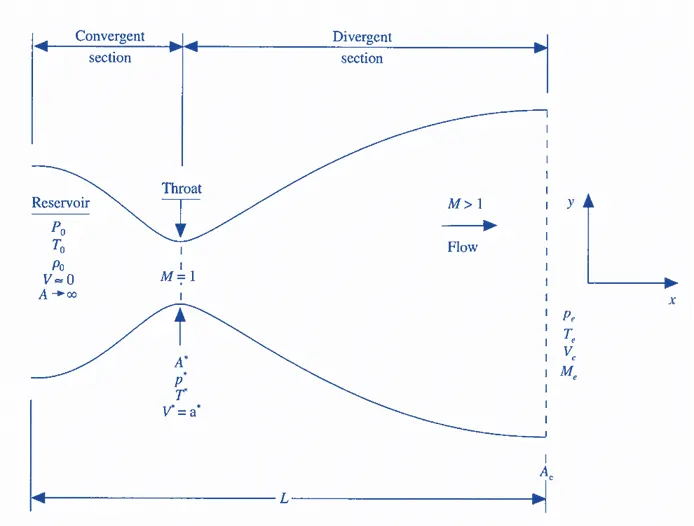
Schematic Diagram of Subsonic-Supersonic Nozzle
(Source: Computational Fluid Dynamics by John D. Anderson)
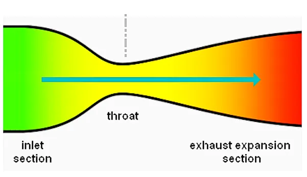
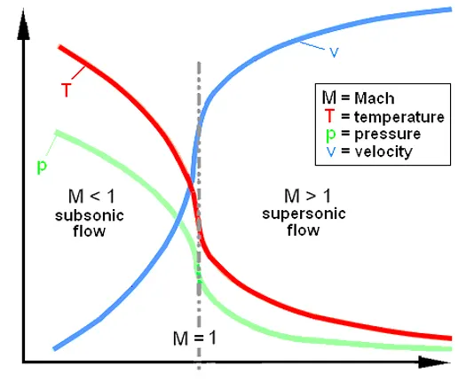
Characteristics of Subsonic-Supersonic Nozzle
Govening Equations -
The Governing Equation For the Quasi One-Dimensional, Steady, Inviscid, Isentropic Flow is as follows,
Continuity Equation - `rho_1*V_1*A_1 =rho_2*V_2*A_2`
Momentum Equation - `p_1*A_1+rho_1*V_(1)^2*A_1+int_(A1)^(A2)p*dA = p_2*A_2+rho_2*V_(2)^2*A_2`
Energy Equation - `h_1+(V_(1)^2)/2 = h_2+(V_(2)^2)/2`
Here, `V` is the Velocity vector, `rho` is the density of the fluid, `A` is Cross-Section Area.
`p` is the pressure, for an Ideal Gas `p = rho*R*T` where, `R` is the Gas Constant & `T` is Temperature.
`h` is the Enthalpy, for an Ideal Gas `h = C_p *T` where, `C_p` is the Specific Heat at Constant Pressure.
MacCormack Method
MacCormack method is a second-order explicit finite difference technique, widely used discretization scheme for the numerical solution of hyperbolic partial differential equations.
It basically consists of 2 steps,
1. Predictor Step -
In this step a provisional value is estimated and discretized for time derivative by forward difference of spatial derivative at time `t + dt`.
2. Corrector Step -
In the corrector step, we again calculate the time derivative at`t+dt`, this time substituting the obtained predicted value in the spatial derivative with backward difference.
Now, the final value is calculated by taking the average of the time derivatives obtained the predictor value and the corrector value.
- The order of differencing is alternative, i.e. can be reversed for the time step (i.e., forward followed by backward, or vise-versa).
- For nonlinear equations, this procedure provides the best results.
- For linear equations, the MacCormack scheme is equivalent to the Lax–Wendroff method.
- Unlike first-order upwind scheme, the MacCormack does not introduce diffusive errors in the solution.
However, it is known to introduce - dispersive errors (Gibbs phenomenon) in the region where the gradient is high.
- The Stability requirement is that the Courant No. be less than 1.
THE CASE AND SIMULATION SETUP -
The Setup -
- Deducing Governing Equations - in Conservation and Non-Conservation Form
- Discretization Method
- Boundary Conditons
- Initial Conditions
- Time Step Calculation
1. THE GOVERNING EQUATIONS
The Case we are dealing in this project is, the Quasi 1-D Invisicid Supersonic Nozzle Flow problem. With simplifying assumption of quasi one-dimensional flow, we assume that the flow properties are uniform across any given cross-secton of the nozzle, in reality the the nozzle flow is 2 dimensional flow, with the change in C/S Area w.r.t x, there will be Flow-Field Variation in both x and y directions. Therefore by this assumption we twisted the real physics. Therefore, to ensure the physical principles are justified with the assumption of Quasi-1-D Flow we are going to derive equations that holds inspite of the twisted physics, by applying the Integral forms of governing equations to a Control Volume which will be consistent with the quasi 1D flow.
a) Integral Forms of the Governing Equations -
Continuity Equation - `del/(delt) intintint_(V) rho*d∀ + del/(delt) intint_(S) rho*V*dS =0`
Momentum Equation - `del/(delt) intintint_(V) (rho.u)*d∀ + del/(delt) intint_(S) (rho.u.V)*dS = - intint_(S) p*dS`
Energy Equation - `del/(delt) intintint_(V) rho*(e+V^2/2)*d∀ + del/(delt) intint_(S) rho*(e+V^2/2).V*dS = - intint_(S) (p.V)*dS`
Here, Since its considered Inviscid Flow therefore the Viscous terms are neglected. It is 1-Dimensional flow at x-direction.
`u` is the fluid velocity component at x - direction, terms of velocity for other directions are neglected.
`e` is the internal energy, for a ideal gas `e = C_v *T` where, `C_v` is the specific heat at constant volume.
`p` is the Pressure and `rho`is the density, for ideal gas `p = rho*R*T` where, `R` is the Gas Constant.
`V` is the Net Velocity Vector, and `∀` is the Control Volume
`dS` is the Area Vector, it is always Normal to the C/S Area or any surface Area.
b) Partial Differential Form of the Governing Equations -
Consider the Control Volume as shown below for deriving the partial differential equations for the our case of Quasi 1-D Nozzle flow -
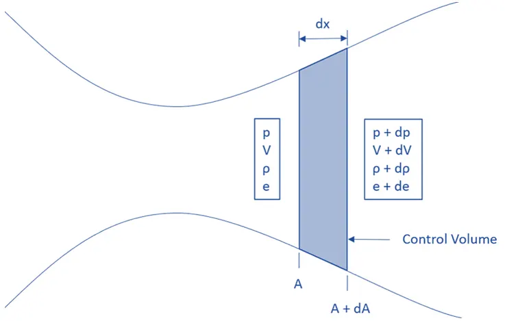
By applying the above Integral form of governing equation this system of control volume we can deduce the Partial Differential Governing Equations for the problem.
Inorder to obtain Momentium equation, following diagram shows the forces acting on the control volume,
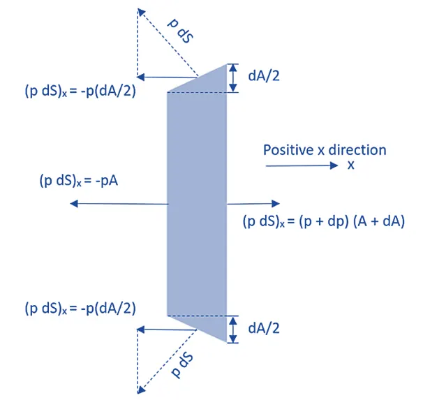
The Forces Acting on the Control Volume Along X - Direction
Following is the Governing Equations for the Quasi 1-D Invisid, Unsteady, Isentropic Subsonic-Supersonic Nozzle Flow -
- Non - Conservation Form (Control Volume is Moving along the fluid)
Continuity Equation - `(del(rhoA))/(delt) + rhoA(delV)/(delx) + rhoV(delA)/(delx) + VA(delrho)/(delx) = 0`
Momentum Equation - `rho(delV)/(delt) + rhoV(delV)/(delt) = -R(rho(delT)/(delx) + T(delrho)/(delx))`
Energy Equation - `rhoC_v(delT)/(delt) + rhoVC_v(delT)/(delx) = - rhoRT((delV)/(delx)+ V(del(lnA))/(delx))`
- Conservation Form (Control Volume is Stationary)
Continuity Equation - `(del(rhoA))/(delt) + (del(rhoAV))/(delx) = 0`
Momentum Equation - `(del(rhoAV))/(delt) + (del(rhoAV^2))/(delx) = -A(delrho)/(delx)`
Energy Equation - `(del(rho.A.(e+V^2/2)))/(delt) + (del(rho.A.V.(e+V^2/2)+pAV))/(delx) = 0`
c) Non-Dimensional Form Partial Differential Governing Equations -
In Fluid Dynamics, Non-dimensionalization of the equations is the conversion of the equations to a nondimensional form. This technique can ease the analysis of the problem at hand, and reduce the number of free parameters. Small or large sizes of certain dimensionless parameters indicate the importance of certain terms in the equations for the studied flow. This may provide possibilities to neglect terms in certain (areas of the) considered flow.
For the Nozzle Flows, the flow field variables are frequently expressed in terms of non-dimensional variables, such that Flow variables are referenced to their reservoir/inlet values.
Non-Dimesional Variable for the governing equation with respect to the Flow-Feild Variables are as follows,
`T' = T/T_o` `rho' = rho/rho_o` `V' = V/a_o` `A' = A/A^star` `x' = x/L` `t' = t/(L/a_o)`
here, `a_o = sqrt(gamma*R*T)`, Speed of Sound at the Reservoir.
`T' =` Non-dimensional Temperature, `T =` Temperature of the fluid, `T_o =` Temperature at the Reservoir
`rho' =` Non-dimensional Density, `rho =` Density of the fluid, `rho_o =` Density at the Reservoir
`V' =` Non-dimensional Velocity, `V =` Velocity of the fluid
`A' =` Non-dimensional Area, `A =` C/S Area of the Nozzle, `A^star =` C/S Area at the Nozzle Throat
`x' =` Non-dimensional Location, `x =` Location in the Nozzle, `L =` Length of the Nozzle
`t' =` Non-dimensional Time, `t =` Time
Non - Dimensional form of the Governing Equations for the Quasi 1-D Nozzle Flow are as follows,
- Non - Conservation Form (Control Volume is Moving along with Fluid Flow)
Continuity Equation - `(delrho')/(delt') = - rho'(delV')/(delx') - rho'V'(del(lnA'))/(delx') - V'(delrho')/(delx')`
Momentum Equation - `(delV')/(delt') = - V'(delV')/(delx') - 1/gamma ((delT')/(delx') + (T')/(rho')*(delrho')/(delx') )`
Energy Equation - `(delT')/(delt') = - V'(delT')/(delx') - (gamma-1).T'( (delV')/(delx') + V'(del(lnA'))/(delx') )`
- Conservation Form (Control Volume is Stationary)
Continuity Equation - `(del(rho'A'))/(delt') + (del(rho'A'V'))/(delx') = 0`
Momentum Equation - `(del(rho'A'V'))/(delt') + (del(rho'A'V'^2 + (1/gamma)p'A'))/(delx') = 1/gamma*p'(delA')/(delx')`
Energy Equation - `(del(rho'.A'.((e')/(gamma-1)+ gamma/2V'^2)))/(delt') + (del(rho'.A'.V'.((e')/(gamma-1)+gamma/2V'^2)+p'A'V'))/(delx') = 0`
Following Simplification of the Conservation Form Governing Equation for the Code,
Continuity Equation - `(delU_1)/(delt') = - (delF_1)/(delx')`
Momentum Equation - `(delU_2)/(delt') = - (delF_2)/(delx') +J_2`
Energy Equation - `(delU_3)/(delt') = - (delF_3)/(delx')`
Here, `U_1 = rho'A'` `F_1 = rho'A'V'`
`U_2 = rho'A'V'` `F_2 = rho'A'V'^2 + (1/gamma)p'A'` `J_2 = 1/gamma*p'(delA')/(delx')`
`U_3 = rho'.A'.((e')/(gamma-1)+ gamma/2V'^2)` `F_3 = rho'.A'.V'.((e')/(gamma-1)+gamma/2V'^2)+p'A'V'`
`rho' = U_1/(A')` `V' = U_2/U_1` `T' = e' = (gamma-1)(U_3/U_1 - gamma/2V'^2)` `p' = rho'T'`
2. DISCRETIZATION
Grid Generation - To implement a finite-difference solution, we divide the Nozzle length into a number of discrete grid points along the X - direction, as shown in the following. We have taken the assumption of Quasi 1-D Nozzle Flow, that means the Flow Variables values at the at centre of a nozzle cross-section will be same and uniform at all points of that cross-section, whether the point be at the centre or along the wall. This assumption of Quasi-1D and Inviscid reduces the complexity for the grid generation, as we can study the flow by create grid at centre/axis of the nozzle , rather than complex profile of the Nozzle wall.
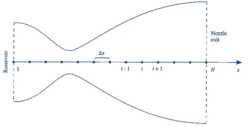
Grid Point Generation along the Nozzle
The Grid points are evenly distributed along the x-axis, with `Deltax` or `dx` denotes the spacing between the grid points.
We are using a MacCormack Technique for the Discretization. The MacCormack's technique is a predictor-corrector method. In the time-marching approach. we know the flow-field variables at the time `t` , and we use the difference equations to solve explicitly for the variables at time `t+Deltat` .
The MacCormack method is as follows,
(a) Predictor Step
- Discretizing the governing equation using the forward difference method. We set the spatial derivatives as foward differences, and calculate the time derivative terms.
- From the time derivates, updating the values of primitive variables.
(b) Corrector Step.
- Discretizing the equations using the backward difference and from the predicted values of the flow variables from the predictor step.
- Computing the average of the time derivatives of governing equations solved by the predictor and corrector method.
- Updating the primitive variable terms and obtaining the final corrected values, by the average time derivatives.
3. BOUNDARY CONDTIONS
Inorder to examine the boundary conditions, we consider Two infinitely weak Mack waves at the boundary points, both proporgating with speed of sound `a` . One proporgating towards left direction and other moving towards right direction, both labeled as 'Left-Running Characteristic' and 'Right-Running Characteristic' Respectively.
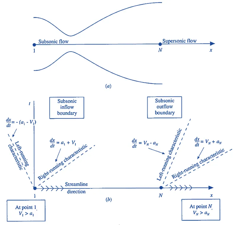
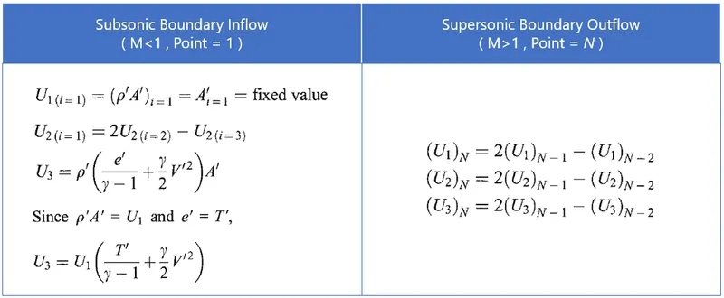
Study of Boundary Conditions : Subsonic Inflow and Supersonic Outflow
Subsonic Inflow Boundary Condition -
From the above figure we can see that at the Subsonic Inlet boundary, lefte running characteristic would be going towards left and the flow coming through inlet which is moving towards right, and will have the subsonic speed. The relative velocity of the left characteristic will `-(a_1-V_1)` and relative velocity for the right running characteristic will be `(a_1+V_1)`. Hence, we can see here that the left running characteristic running characteristic is proporgating out of the nozzle region i.e. outside the domain of influence and right running characteristic proporgates inside the domain.
Therefore, as a conclusion, at the subsonic inlow boundary, we most stipulate the value of Two Fixed Flow-Field Variables that are independent of time, wheres the value of One other variable must be alowed to Float.
So, for the subsonic inlow boundary, we choose that the Density and the Energy Terms to be stipulated. And the Velocity term to be allowed to float with respect to time. The Velocity at the inlet boundary can be estimated by Linear Extrapolation, from the velocities obtained at inner nodes at every time step.
Supersonic Outflow Boundary Condition -
Now, by applying the same concept at the outflow boundary. The fluid flow is flowing towards right direction same as above, however now the speed of the stream is supersonic. So, the relative velocity of left characteristic = `V_N-a_N` and right characteristic = `V_N+a_N` , both dominated dominated by the speed of the fluid flow. Hence, both of the characteristics are proporgating towards right diretion, and i.e. out of the Domain.
Therefore, at the Supersonic Outflow Boundary, since both the characteristic and the stream is going of the domain, So there are no Flow-Field Variables which require their values to be stipulates at the outflow boundary, Hence all variables must be allowed to Float at this boundary.
Here, at the outflow boundary all variables must be allowed to float, therefore we will calculate the variables using the Linear Extrapolation at every time Step.
The Boundary conditions for Quasi 1-D Invisid, Unsteady, Isentropic Subsonic-Supersonic Nozzle Flow -
- Non - Conservation Form
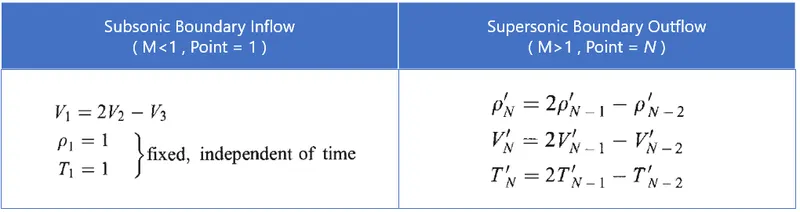
- Conservation Form
4. INITIAL CONDITIONS
Nozzle Shape -
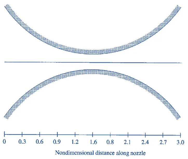
The nozzle shape, `A=A(x)`, is specified and held fixed, independent of time. For the case the parabolic area distribution given by
`A = 1 + 2.2 (x -1.5)^2` `0 le x le 3`0≤x≥3">
Note that `x = 1.5` is the throat of the nozzle, that the convergent section occurs for `x<1.5` and that the divergent section occurs for `x>1.5`. This nozzle shape is as shown in the following figure,
Initial Conditions -
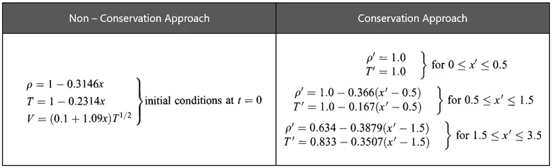
To start the simulation, we have to stipulate the initial conditions for the `rho, T and V` as a function of x, at time `t = 0`. There are two reasons why the choosing of initial conditions should be done carefully.
- The closer the closer theinitial conditions are to the final Steady-State result, the faster the time-marching procedure will converge, and hence, computer execution time will be shorter.
- If the initial Conditions are too far away from the reality, the inital time wise gradients(time derivatives) can become huge at earlt timesteps. These large gradients at the early part of Time-Stepping can cause system to go unstable.
In the current case, we know that `rho` & `T` decreases and V increases as the flow expands through the Nozzle. therefore, we have taken the initial condition that qualitatively beahaves in same fashion. The initial condions with the linear variations of the flow-feild variables as the function of `x` is as follows,
5. TIME STEP CALCULATION
We can see our governing equations are hyperbolic and we will be using explicit methods to solve it, and hence computing the timestep is very critical as explicit time-integration method is sensitive to timestep. Having a wrong timestep will blow up our solution in no time thereby making our solution unstable, illogical and unusable. Therefore, we shall be using the Courant number to calculate the Time Step Size for a stable solution.
This is known as adaptive time step. Inorder to avoid the solution to blow-up the Time-Step Size should be calculated at every timestep loop from the Courant no. For the our problem we will consider C = 0.5 for the optimum solution.
`triangle t = dt = min(C*dx/(a+v))`
In Non-Dimensional Form,
Non-Dimensional velocity of sound, `a' = a/a_o` Non-Dimensional Velocity, `v' = v/a_o`
`dt = min(C*dx/(a'+v'))`
where, `a =`Local Velocity of sound
`a_o =`Velocity of sound
`v =` Velocity of the fluid
`a' =`Non-Dimensional Velocity of sound
`v' =`Non-Dimensional Velocity of fluid
Now, `a' = a/a_o = sqrt(gamma.R.T)/sqrt(gamma.R.T_o) = sqrt(T/T_o) = sqrt(T') = (T')^(1/2)`
`implies` ` dt = min(C*dx/((T')^(1/2)+v'))`
PROGRAM -
The Following is the Main Function of the Program -
% ------------------------- Mid Term Project -  Quasi 1-D Supersonic Nozzle Analysis by using MacCormack Method  -------------------------

clear all;
close all;
clc;

fprintf('nttttttt Quasi 1-D Supersonic Nozzle Analysis by using MacCormack Method');

% Inputs for the quasi 1D nozzle flow simulation

L = 3;                  % Domain Length
n = input('nn     Enter the No. of Nodes or Grid Size [Recommended 31 or 61]) : ');                 % Number of grid points along x direction in array form
x = linspace(0,3,n);
dx = x(2)-x(1);
gama = 1.4;            % Ratio of specific heats (Cp/Cv) for air at standard conditions

% Nozzle Shape
a = 1+2.2*(x-1.5).^2;   % Area
b = a.*(-1);
n_throat = find(a==1);

nt = 1400;      % Number of time steps
cfl = 0.5;      % Courant numbe5r initialisation

 filename = sprintf('Results %d Nodes',n);
 path = ('D:Super Sonic Nozzle');
 mkdir(path,filename);                     % mkdir() is used create New folder

% -----------------------------------------------------------------------------------------
%                                  Analytical Calculation
% -----------------------------------------------------------------------------------------

M = 0;
% Mach Number
for i = 1:round(n/2)        % From Inlet to Throat
    resi = 1;
    while resi > 1e-9
        M = M + 1e-4;
        resi = ((1/M^2)*((2/(gama+1))*(1+((gama-1)/2)*M^2))^((gama+1)/(gama-1)))-(a(i)^2);
    end
    M_e(i) = M;
end

for i = round(n/2):n        % From Throat to Outlet
    resi = 1;
    while resi > 1e-9
        M = M + 1e-4;
        resi = ((1/M^2)*((2/(gama+1))*(1+((gama-1)/2)*M^2))^((gama+1)/(gama-1)))-(a(i)^2);
        resi = resi*(-1);
    end
    M_e(i) = M;
end

rho_e = (1+(((gama-1)/2).*M_e.^2)).^(-1/(gama-1));
T_e = (1+(((gama-1)/2).*(M_e.^2))).^(-1);
p_e = rho_e.*T_e;
mfr_e = ones(n).*0.579;

% Plotting the Exact Analytical Solution
figure1 = figure('position',[50 -30 750 1200]);
subplot(5,1,1)
    sgtitle('Analytical Solution','color',[0.1,0.1,0.6],'color',[0.1,0.1,0.4]);
    plot(x,a,'color',[0.8 0.1 0.1],'linewidth',1.5);
    title('Supersonic Nozzle Profile along X-Direction')
    hold on;
    plot(x,b,'color',[0.9 0.1 0.1],'linewidth',1.5);
    plot([x(round(n/2)) x(round(n/2))],[-5 5],':','color','k');
subplot(5,1,2)
    plot(x,M_e,'-o','color',[0.85 0.3 0.1],'linewidth',1.5,'MarkerSize',2,'MarkerEdgeColor',[0.5 0.2 0.2],'MarkerFaceColor',[0.85 0.3 0.1]);
    title('Mach Number vs  x / L');
    grid on;
    xlabel('x / L');    ylabel('M');
subplot(5,1,3)
    plot(x,p_e,'-o','color',[0.85 0.3 0.1],'linewidth',1.5,'MarkerSize',2,'MarkerEdgeColor',[0.5 0.2 0.2],'MarkerFaceColor',[0.85 0.3 0.1]);
    title('Pressure Ratio vs  x / L');
    grid on;
    xlabel('x / L');    ylabel('P/Po');
subplot(5,1,4)
    plot(x,rho_e,'-o','color',[0.85 0.3 0.1],'linewidth',1.5,'MarkerSize',2,'MarkerEdgeColor',[0.5 0.2 0.2],'MarkerFaceColor',[0.85 0.3 0.1]);
    title('Density Ratio vs  x / L');
    grid on;
    xlabel('x / L');    ylabel('ρ/ρo');
subplot(5,1,5)
    plot(x,T_e,'-o','color',[0.85 0.3 0.1],'linewidth',1.5,'MarkerSize',2,'MarkerEdgeColor',[0.5 0.2 0.2],'MarkerFaceColor',[0.85 0.3 0.1]);
    title('Temperature Ratio vs  x / L');
    grid on;
    xlabel('x / L');    ylabel('T/To');

p1 = fullfile(path,filename,'1.Analytical Solution.png');
saveas(figure1,p1);


% -----------------------------------------------------------------------------------------
%                                  Non-Conservative Form
% -----------------------------------------------------------------------------------------

% Initial Conditions for Non-Conservative form
rho_nc = 1-0.3146*x;
T_nc = 1-0.2314*x;
v_nc = (0.1+1.09*x).*T_nc.^0.5;
p_nc = rho_nc.*T_nc;
mf_nc = rho_nc.*v_nc.*a;
M_nc = v_nc./(T_nc.^0.5);

figure2 = figure('position',[50 70 1366 720]);
ct = 1;
time_nc = 0;

for i = 1:nt        % Time Loop

    tic;
    %dt_nc = min((cfl*dx)./(a+v_nc));
    dt_nc = min(cfl*(dx./(v_nc+(T_nc.^(0.5)))));

    rho_old = rho_nc;
    v_old = v_nc;
    T_old = T_nc;
    M_old = M_nc;
    p_old = p_nc;

    % Predictor method

    for j = 2:n-1

        dvdx = (v_nc(j+1)-v_nc(j))/dx;
        drhodx = (rho_nc(j+1)-rho_nc(j))/dx;
        dTdx = (T_nc(j+1)-T_nc(j))/dx;
        dlogadx = (log(a(j+1))-log(a(j)))/dx;

        % Continuty Equation
        drhodt_p(j) = -rho_nc(j)*dvdx-rho_nc(j)*v_nc(j)*dlogadx - v_nc(j)*drhodx;

        % Momentum Equation
        dvdt_p(j) = -v_nc(j)*dvdx-(1/gama)*(dTdx + (T_nc(j)/rho_nc(j))*drhodx);

        % Energy Equation
        dTdt_p(j) = -v_nc(j)*dTdx - ((gama-1)*T_nc(j))*(dvdx + v_nc(j)*dlogadx);

        % solution update
        rho_nc(j) = rho_nc(j) + drhodt_p(j)*dt_nc;
        v_nc(j) = v_nc(j) + dvdt_p(j)*dt_nc;
        T_nc(j) = T_nc(j) + dTdt_p(j)*dt_nc;

    end


    % Corrector method
    for j = 2:n-1

        dvdx = (v_nc(j)-v_nc(j-1))/dx;
        drhodx = (rho_nc(j)-rho_nc(j-1))/dx;
        dTdx = (T_nc(j)-T_nc(j-1))/dx;
        dlogadx = (log(a(j))-log(a(j-1)))/dx;

        % Continuty equation
        drhodt_c(j) = -rho_nc(j)*dvdx - rho_nc(j)*v_nc(j)*dlogadx - v_nc(j)*drhodx;

        % Momentum equation
        dvdt_c(j) = -v_nc(j)*dvdx - (1/gama)*(dTdx + (T_nc(j)/rho_nc(j))*drhodx);

        % Energy Equation
        dTdt_c(j) = -v_nc(j)*dTdx - (gama-1)*T_nc(j)*(dvdx + v_nc(j)*dlogadx);

    end


    % Compute the average time derivative
    drhodt_nc = 0.5*(drhodt_p + drhodt_c);
    dvdt_nc = 0.5*(dvdt_p + dvdt_c);
    dTdt_nc = 0.5*(dTdt_p + dTdt_c);


    % final solution Update
    for k = 2:n-1
        rho_nc(k) = rho_old(k) + drhodt_nc(k)*dt_nc;
        v_nc(k) = v_old(k) + dvdt_nc(k)*dt_nc;
        T_nc(k) = T_old(k) + dTdt_nc(k)*dt_nc;
    end


    % Apply the boundary conditions
    % Inlet
    v_nc(1) = 2*v_nc(2) - v_nc(3);

    % Outlet
    v_nc(n) = 2*v_nc(n-1) - v_nc(n-2);
    rho_nc(n) = 2*rho_nc(n-1) - rho_nc(n-2);
    T_nc(n) = 2*T_nc(n-1) - T_nc(n-2);

    % Pressure
    p_nc = rho_nc.*T_nc;

    % Mass Flow rate
    mfr_nc = rho_nc.*a.*v_nc;

    % Mach Number
    M_nc = v_nc./(T_nc.^0.5);


    if i==50
        nmfr_nc(1,:) = rho_nc.*v_nc.*a;
        nmfr_nc_nt(1) = i;
    elseif i==100
        nmfr_nc(2,:) = rho_nc.*v_nc.*a;
        nmfr_nc_nt(2) = i;
    elseif i==150
        nmfr_nc(3,:) = rho_nc.*v_nc.*a;
        nmfr_nc_nt(3) = i;
    elseif i==200
        nmfr_nc(4,:) = rho_nc.*v_nc.*a;
        nmfr_nc_nt(4) = i;
    elseif i==700
        nmfr_nc(5,:) = rho_nc.*v_nc.*a;
        nmfr_nc_nt(5) = i;
    elseif i==1400
        nmfr_nc(6,:) = rho_nc.*v_nc.*a;
        nmfr_nc_nt(6) = i;
    end

    % Residual and convergance analysis by the values at the Nozzle throat

    err_rho_nc = abs(rho_old(n_throat)-rho_nc(n_throat));
    err_upd_rho_nc(1,i) = err_rho_nc;
    err_v_nc = abs(v_old(n_throat)-v_nc(n_throat));
    err_upd_v_nc(1,i) = err_v_nc;
    err_T_nc = abs(T_old(n_throat)-T_nc(n_throat));
    err_upd_T_nc(1,i) = err_T_nc;
    err_M_nc = abs(M_old(n_throat)-M_nc(n_throat));
    err_upd_M_nc(1,i) = err_M_nc;
    err_p_nc = abs(p_old(n_throat)-p_nc(n_throat));
    err_upd_p_nc(1,i) = err_p_nc;

    rho_nc_t(1,i) = rho_nc(n_throat);
    v_nc_t(1,i) = v_nc(n_throat);
    T_nc_t(1,i) = T_nc(n_throat);
    M_nc_t(1,i) = M_nc(n_throat);
    p_nc_t(1,i) = p_nc(n_throat);

    time_nc = time_nc + toc;

    tsr = 1:i;   % Timestep range in array corresponding to current timestep
    titletext = sprintf(' Time = %.4f s                 No. of Nodes = %d',dt_nc*i,n);

    % Plotting the time-wise variation/convergence of non-dimensional characteristic variables
    if rem(i,20) == 0
        subplot(4,2,2)
        plot(tsr,rho_nc_t,'color',[0.4,0.4,0.4],'linewidth',1.5);
        title("Timewise Variation of Non-Dimensional Density at Nozzle Throat")
        xlabel('No. of Time Steps');    ylabel('ρ/ρo');
        grid on; hold on;

        subplot(4,2,4)
        plot(tsr,T_nc_t,'color',[0.4,0.4,0.4],'linewidth',1.5);
        title("Timewise Variation of Non-Dimensional Temperature at Nozzle Throat")
        xlabel('No. of Time Steps');    ylabel('T/To');
        grid on; hold on;

        subplot(4,2,6)
        plot(tsr,p_nc_t,'color',[0.4,0.4,0.4],'linewidth',1.5);
        title("Timewise Variation of Non-Dimensional Pressure at Nozzle Throat")
        xlabel('No. of Time Steps');    ylabel('P/Po');
        grid on; hold on;

        subplot(4,2,8)
        plot(tsr,M_nc_t,'color',[0.4,0.4,0.4],'linewidth',1.5);
        title('Timewise Variation of Mach number at Nozzle Throat')
        xlabel('No. of Time Steps');    ylabel('M');
        grid on; hold on;

        subplot(4,2,[1,3,5,7])
        residual_err_plot = semilogy(tsr,err_upd_rho_nc,tsr,err_upd_v_nc,tsr,err_upd_T_nc,tsr,err_upd_p_nc,tsr,err_upd_M_nc);
        set(residual_err_plot(1), 'color', [0.85 0.8 0.1],'linewidth',1.5);
        set(residual_err_plot(2), 'color', [0 0.9 0.9],'linewidth',1.5);
        set(residual_err_plot(3), 'color', [0.85 0.1 0.1],'linewidth',1.5);
        set(residual_err_plot(4), 'color', [0.8 0.2 0.6],'linewidth',1.5);
        set(residual_err_plot(5), 'color', [0.3 0.8 0.2],'linewidth',1.5);
        title(sprintf("Residual w.r.t No. of Time steps at nozzle throat"),titletext)
        ylabel('Residual');       xlabel('No. of Time Steps');
        grid on; hold on;
        l_text1 = sprintf('Density');
        l_text2 = sprintf('Velocity');
        l_text3 = sprintf('Temperature');
        l_text4 = sprintf('Pressure');
        l_text5 = sprintf('Mach number');

        legend(l_text1,l_text2,l_text3,l_text4,l_text5);
        sgtitle('Analyzing Convergence of the Charateristic Variables at the Nozzle Throat for Non-Conservation Approach','color',[0.1,0.1,0.4],'FontWeight','bold');

        pause(0.03)
        M1(ct) = getframe(gcf);
        ct = ct+1;
    end

end


 p2 = fullfile(path,filename,sprintf('2.Observing Convergence at throat by Non-Conservation, %d Nodes.png',n));
 saveas(figure2,p2);

 movie(M1);   % Play recorded movie frames
 text = sprintf('Analysis At throat by Non-Conservation, %d Nodes .avi',n);
 video = VideoWriter(text,'Motion JPEG AVI');
 open(video);            % Open file for writing video data
 writeVideo(video,M1);    % Write video data to file
 close(video);           % Close file after writing video data

% Results of Non-Conservation Method
figure3 = figure('position',[50 -30 750 1200]);
subplot(5,1,1)
    sgtitle('Numerical Solution by Non-Conservation Approach','color',[0.1,0.1,0.4]);
    plot(x,a,'color',[0.8 0.1 0.1],'linewidth',1.5);
    title('Supersonic Nozzle Profile along X-Direction')
    hold on;
    plot(x,b,'color',[0.9 0.1 0.1],'linewidth',1.5);
    plot([x(round(n/2)) x(round(n/2))],[-5 5],':','color','k');
    plot(x,0,'--ko','MarkerSize',2,'MarkerEdgeColor','k','MarkerFaceColor',[0.7,0.7,0.7]);
    plot([x(1) x(n)],[0 0],':','color','k')
subplot(5,1,2)
    plot(x,M_nc,'color',[0.2 0.2 0.9],'linewidth',1.5);
    title('Mach Number vs  x / L');
    grid on;
    xlabel('x / L');    ylabel('M');
subplot(5,1,3)
    plot(x,p_nc,'color',[0.2 0.2 0.9],'linewidth',1.5);
    title('Pressure Ratio vs  x / L');
    grid on;
    xlabel('x / L');    ylabel('P/Po');
subplot(5,1,4)
    plot(x,rho_nc,'color',[0.2 0.2 0.9],'linewidth',1.5);
    title('Density Ratio vs  x / L');
    grid on;
    xlabel('x / L');    ylabel('ρ/ρo');
subplot(5,1,5)
    plot(x,T_nc,'color',[0.2 0.2 0.9],'linewidth',1.5);
    title('Temperature Ratio vs  x / L');
    grid on;
    xlabel('x / L');    ylabel('T/To');

p3 = fullfile(path,filename,'3.Numerical Solution by Non-Conservation.png');
saveas(figure3,p3);


% Plotting Non-Dimensional Mass Flow rate at different No. of Time Steps For Non-Conservation Method
figure4 = figure('position',[50 -30 640 480]);
for q = 1:6
    plot(x,nmfr_nc(q,:),'linewidth',1.5);
    hold on;
end
title('Non-Dimensional Mass Flow rate at different No. of Time Steps','For Non-Conservation Method');
grid on;    hold on;    xlabel('x / L');    ylabel('ρ*A*V / ρo*A*Vo');
plot(x,mfr_e,'-o','color',[0.85 0.3 0.1],'linewidth',1.5,'MarkerSize',2,'MarkerEdgeColor',[0.5 0.2 0.2],'MarkerFaceColor',[0.85 0.3 0.1]);
l_text1 = sprintf('%d Time Steps',nmfr_nc_nt(1));
l_text2 = sprintf('%d Time Steps',nmfr_nc_nt(2));
l_text3 = sprintf('%d Time Steps',nmfr_nc_nt(3));
l_text4 = sprintf('%d Time Steps',nmfr_nc_nt(4));
l_text5 = sprintf('%d Time Steps',nmfr_nc_nt(5));
l_text6 = sprintf('%d Time Steps',nmfr_nc_nt(6));
l_text7 = sprintf('Exact/Analytical Value (%.3f)',mfr_e(1));
legend(l_text1,l_text2,l_text3,l_text4,l_text5,l_text6,l_text7);

p4 = fullfile(path,filename,'4.Mass Flow rate at No. of TimeSteps For Non-Conservation.png');
saveas(figure4,p4);


% -----------------------------------------------------------------------------------------
%                                  Conservativation Form
% -----------------------------------------------------------------------------------------

% Initial Conditions for Conservative form
for i = 1:length(x)

    if x(i)<=0.5
        rho_c(i)=1;
        T_c(i)=1;

    elseif x(i)>=0.5 && x(i)<=1.5
        rho_c(i) = 1-0.366*(x(i)-0.5);
        T_c(i) = 1-0.167*(x(i)-0.5);

    elseif x(i)>=1.5 && x(i)<=3
        rho_c(i) = 0.634-0.3879*(x(i)-1.5);
        T_c(i) = 0.833-0.3507*(x(i)-1.5);
    end
end
v_c = 0.59./(rho_c.*a);
p_c = rho_c.*T_c;
mf_c = rho_c.*v_c.*a;
M_c = v_c./(T_c.^0.5);

% Initializing solution terms
U1 = rho_c.*a;
U2 = rho_c.*a.*v_c;
U3 = U1.*((T_c/(gama-1))+(gama/2).*(v_c.^2));

J2_p = ones(1,n);
J2_c = ones(1,n);

figure5 = figure('position',[50 70 1366 720]);
ct = 1;
time_c = 0;

for i = 1:nt

    tic;

    %dt_c = min((cfl*dx)./(a+v_c));
    dt_c = min(cfl*(dx./(v_c+(T_c.^(0.5)))));

    U1_old = U1;
    U2_old = U2;
    U3_old = U3;
    rho_old = rho_c;
    v_old = v_c;
    T_old = T_c;

    %F1 = U2;
    %F2 = U2.*(v_c) + (U1/gama);
    %F3 = U3.*(v_c) + U2;
    F1 = U2;
    F2 = (((U2.^2)./U1)+(((gama-1)/gama).*(U3 - ((gama/2)*((U2.^2)./U1)))));
    F3 = (((gama.*U2.*U3)./U1)-((((gama*(gama-1))/2))*((U2.^3)./U1.^2)));

    % Predictor Step
    for j = 2:n-1

        dadt_p(j) = (a(j+1) - a(j))/dx;
        J2_p(j) = (1/gama).*(rho_c(j)).*(T_c(j)).*(dadt_p(j));

        % Continuty Equation
        dU1dt_p(j) = -(F1(j+1) - F1(j))/dx;

        % Momentum Equation
        dU2dt_p(j) = -(F2(j+1) - F2(j))/dx + J2_p(j);

        % Energy Equation
        dU3dt_p(j) = -(F3(j+1) - F3(j))/dx;


        % solution update
        U1(j) = U1(j) + dU1dt_p(j)*dt_c;
        U2(j) = U2(j) + dU2dt_p(j)*dt_c;
        U3(j) = U3(j) + dU3dt_p(j)*dt_c;

    end

    rho_c = U1./a;
    T_c = (gama-1) .*( (U3./U1) - ((gama/2).*(v_c).^2) );

    F1 = U2;
    F2 = (((U2.^2)./U1)+(((gama-1)/gama).*(U3 - ((gama/2)*((U2.^2)./U1)))));
    F3 = (((gama.*U2.*U3)./U1)-((((gama*(gama-1))/2))*((U2.^3)./U1.^2)));

    % Corrector method
    for j = 2:n-1

        dadt_c(j) = (a(j) - a(j-1))/dx;
        J2_c(j) = (1/gama).*(rho_c(j)).*(T_c(j)).*dadt_c(j);

        % Continuty Equation
        dU1dt_c(j) = -(F1(j) - F1(j-1))/dx;

        % Momentum Equation
        dU2dt_c(j) = -(F2(j) - F2(j-1))/dx + J2_c(j);

        % Energy Equation
        dU3dt_c(j) = -(F3(j) - F3(j-1))/dx;

    end


    % Compute the average time derivative
    dU1dt = 0.5*(dU1dt_p + dU1dt_c);
    dU2dt = 0.5*(dU2dt_p + dU2dt_c);
    dU3dt = 0.5*(dU3dt_p + dU3dt_c);


    % Final Solution Update
    for k = 2:n-1

        U1(k) = U1_old(k) + dU1dt(k)*dt_c;
        U2(k) = U2_old(k) + dU2dt(k)*dt_c;
        U3(k) = U3_old(k) + dU3dt(k)*dt_c;

    end


    % Updating Boundary Conditions by Extrapolating

    % Inlet
    U1(1) = rho_c(1).*a(1);
    U2(1) = 2*U2(2)-U2(3);
    U3(1) = U1(1)*((T_c(1)/(gama-1))+((gama/2)*(v_c(1)^2)));
    % Outlet
    U1(n) = 2*U1(n-1) - U1(n-2);
    U2(n) = 2*U2(n-1) - U2(n-2);
    U3(n) = 2*U3(n-1) - U3(n-2);

    % Recomputing Characteristic Variables
    rho_c = U1./a;
    v_c = U2./U1;
    T_c = (gama-1).*( (U3./U1) - ((gama/2).*(v_c).^2) );

    % Pressure
    p_c = rho_c.*T_c;

    % Mass Flow rate
    mfr_c = (rho_c).*(v_c).*(a);

    % Mach Number
    M_c = (v_c)./(T_c.^0.5);


    if i==50
        nmfr_c(1,:) = rho_c.*v_c.*a;
        nmfr_c_nt(1) = i;
    elseif i==100
        nmfr_c(2,:) = rho_c.*v_c.*a;
        nmfr_c_nt(2) = i;
    elseif i==150
        nmfr_c(3,:) = rho_c.*v_c.*a;
        nmfr_c_nt(3) = i;
    elseif i==200
        nmfr_c(4,:) = rho_c.*v_c.*a;
        nmfr_c_nt(4) = i;
    elseif i==700
        nmfr_c(5,:) = rho_c.*v_c.*a;
        nmfr_c_nt(5) = i;
    elseif i==1400
        nmfr_c(6,:) = rho_c.*v_c.*a;
        nmfr_c_nt(6) = i;
    end

    % Residual and convergance analysis by the values at the Nozzle throat

    err_rho_c = abs(rho_old(n_throat)-rho_c(n_throat));
    err_upd_rho_c(1,i) = err_rho_c;
    err_v_c = abs(v_old(n_throat)-v_c(n_throat));
    err_upd_v_c(1,i) = err_v_c;
    err_T_c = abs(T_old(n_throat)-T_c(n_throat));
    err_upd_T_c(1,i) = err_T_c;
    err_M_c = abs(M_old(n_throat)-M_c(n_throat));
    err_upd_M_c(1,i) = err_M_c;
    err_p_c = abs(p_old(n_throat)-p_c(n_throat));
    err_upd_p_c(1,i) = err_p_c;

    rho_c_t(1,i) = rho_c(n_throat);
    v_c_t(1,i) = v_c(n_throat);
    T_c_t(1,i) = T_c(n_throat);
    M_c_t(1,i) = M_c(n_throat);
    p_c_t(1,i) = p_c(n_throat);

    time_c = time_c + toc;

    tsr = 1:i;   % Timestep range in array corresponding to current timestep
    titletext = sprintf(' Time = %.4f s                 No. of Nodes = %d',dt_nc*i,n);

    % Plotting the time-wise variation/convergence of non-dimensional characteristic variables
    if rem(i,20) == 0
        subplot(4,2,2)
        plot(tsr,rho_c_t,'color',[0.4,0.4,0.4],'linewidth',1.5);
        title("Timewise Variation of Non-Dimensional Density at Nozzle Throat")
        xlabel('No. of Time Steps');    ylabel('ρ/ρo');
        grid on; hold on;

        subplot(4,2,4)
        plot(tsr,T_c_t,'color',[0.4,0.4,0.4],'linewidth',1.5);
        title('Timewise variation of non-dimensional temperature at nozzle throat')
        xlabel('No. of Time Steps');    ylabel('T/To');
        grid on; hold on;

        subplot(4,2,6)
        plot(tsr,p_c_t,'color',[0.4,0.4,0.4],'linewidth',1.5);
        title('Timewise variation of non-dimensional pressure at nozzle throat')
        xlabel('No. of Time Steps');    ylabel('P/Po');
        grid on; hold on;

        subplot(4,2,8)
        plot(tsr,M_c_t,'color',[0.4,0.4,0.4],'linewidth',1.5);
        title('Timewise variation of Mach number at nozzle throat')
        xlabel('No. of Time Steps');    ylabel('M');
        grid on; hold on;

        subplot(4,2,[1,3,5,7])
        residual_err_plot = semilogy(tsr,err_upd_rho_c,tsr,err_upd_v_c,tsr,err_upd_T_c,tsr,err_upd_p_c,tsr,err_upd_M_c);
        set(residual_err_plot(1), 'color', [0.85 0.8 0.1],'linewidth',1.5);
        set(residual_err_plot(2), 'color', [0 0.9 0.9],'linewidth',1.5);
        set(residual_err_plot(3), 'color', [0.85 0.1 0.1],'linewidth',1.5);
        set(residual_err_plot(4), 'color', [0.8 0.2 0.6],'linewidth',1.5);
        set(residual_err_plot(5), 'color', [0.3 0.8 0.2],'linewidth',1.5);
        title(sprintf("Residual w.r.t No. of Time steps at nozzle throat"),titletext)
        xlabel('No. of Time Steps');    ylabel('Residual');
        grid on; hold on;
        l_text1 = sprintf('Density');
        l_text2 = sprintf('Velocity');
        l_text3 = sprintf('Temperature');
        l_text4 = sprintf('Pressure');
        l_text5 = sprintf('Mach number');

        legend(l_text1,l_text2,l_text3,l_text4,l_text5);
        sgtitle('Analyzing Convergence of the Charateristic Variables at the Nozzle Throat for Conservation Approach','color',[0.1,0.1,0.4],'FontWeight','bold');

        pause(0.03)
        M2(ct) = getframe(gcf);
        ct = ct+1;
    end

end


 p5 = fullfile(path,filename,sprintf('5.Observing Convergence at throat by Conservation, %d Nodes.png',n));
 saveas(figure5,p5);

 movie(M2);   % Play recorded movie frames
 text = sprintf('Analysis At throat by Conservation, %d Nodes .avi',n);
 video = VideoWriter(text,'Motion JPEG AVI');
 open(video);            % Open file for writing video data
 writeVideo(video,M2);    % Write video data to file
 close(video);           % Close file after writing video data


% Results of Conservation Method
figure6 = figure('position',[50 -30 750 1200]);
subplot(5,1,1)
    sgtitle('Numerical Solution by Conservation Approach','color',[0.1,0.1,0.4]);
    plot(x,a,'color',[0.8 0.1 0.1],'linewidth',1.5);
    title('Supersonic Nozzle Profile along X-Direction')
    hold on;
    plot(x,b,'color',[0.9 0.1 0.1],'linewidth',1.5);
    plot([x(round(n/2)) x(round(n/2))],[-5 5],':','color','k');
    plot(x,0,'--ko','MarkerSize',2,'MarkerEdgeColor','k','MarkerFaceColor',[0.7,0.7,0.7]);
    plot([x(1) x(n)],[0 0],':','color','k')
subplot(5,1,2)
    plot(x,M_c,'color',[0.2 0.75 0.2],'linewidth',1.5);
    title('Mach Number vs  x / L');
    grid on;
    xlabel('x / L');    ylabel('M');
subplot(5,1,3)
    plot(x,p_c,'color',[0.2 0.75 0.2],'linewidth',1.5);
    title('Pressure Ratio vs  x / L');
    grid on;
    xlabel('x / L');    ylabel('P/Po');
subplot(5,1,4)
    plot(x,rho_c,'color',[0.2 0.75 0.2],'linewidth',1.5);
    title('Density Ratio vs  x / L');
    grid on;
    xlabel('x / L');    ylabel('ρ/ρo');
subplot(5,1,5)
    plot(x,T_c,'color',[0.2 0.75 0.2],'linewidth',1.5);
    title('Temperature Ratio vs  x / L');
    grid on;
    xlabel('x / L');    ylabel('T/To');

p6 = fullfile(path,filename,'6.Numerical Solution by Conservation.png');
saveas(figure6,p6);

% Plotting Non-Dimensional Mass Flow rate at different No. of Time Steps For Conservation Method
figure7 = figure('position',[50 -30 640 480]);
    for q = 1:6
        plot(x,nmfr_c(q,:),'linewidth',1.5)
        hold on
    end
    title('Non-Dimensional Mass Flow rate at different No. of Time Steps','For Conservation Method');
    grid on;    hold on;    xlabel('x / L');    ylabel('ρ*A*V / ρo*A*Vo');
    plot(x,mfr_e,'-o','color',[0.85 0.3 0.1],'linewidth',1.5,'MarkerSize',2,'MarkerEdgeColor',[0.5 0.2 0.2],'MarkerFaceColor',[0.85 0.3 0.1]);
    l_text1 = sprintf('%d Time Steps',nmfr_c_nt(1));
    l_text2 = sprintf('%d Time Steps',nmfr_c_nt(2));
    l_text3 = sprintf('%d Time Steps',nmfr_c_nt(3));
    l_text4 = sprintf('%d Time Steps',nmfr_c_nt(4));
    l_text5 = sprintf('%d Time Steps',nmfr_c_nt(5));
    l_text6 = sprintf('%d Time Steps',nmfr_c_nt(6));
    l_text7 = sprintf('Exact/Analytical Value (%.3f)',mfr_e(1));
    legend(l_text1,l_text2,l_text3,l_text4,l_text5,l_text6,l_text7);
p7 = fullfile(path,filename,'7.Mass Flow rate at No. of TimeSteps For Conservation.png');
saveas(figure7,p7);

% Comparison of Non-Dimensional Mass Flow rate throughout the Nozzle
figure8 = figure('position',[80 60 640 480]);
    plot(x,mfr_nc,'color',[0.2 0.2 0.9],'linewidth',1.5);
    title('Comparison of Non-Dimensional Mass Flow rate throughout the Nozzle');
    grid on;    hold on;
    xlabel('x / L');    ylabel('ρ*A*V / ρo*A*Vo');
    axis([0 x(n) 0.57 0.59])
    plot(x,mfr_c,'color',[0.2 0.75 0.2],'linewidth',1.5);
    plot(x,mfr_e,'-o','color',[0.85 0.3 0.1],'linewidth',1.5,'MarkerSize',2,'MarkerEdgeColor',[0.5 0.2 0.2],'MarkerFaceColor',[0.85 0.3 0.1]);
    legend('Non-Conservation Method','Conservation Method','Exact/Analytical Solution','Location','northwest')
p8 = fullfile(path,filename,'8.Comparison of Non-Dimensional Mass Flow rate.png');
saveas(figure8,p8);


% Comparison of the Solution profile of all the methods
figure9 = figure('position',[50 -30 850 1200]);
    sgtitle('Solution Comparison between Analytical vs Non-Conservation Method vs Conservation Method','color',[0.1,0.1,0.4]);
    subplot(5,1,1)
    plot(x,M_nc,'color',[0.2 0.2 0.9],'linewidth',1.5);
    title('Mach Number vs  x / L');
    grid on;    hold on;
    xlabel('x / L');    ylabel('M');
    plot(x,M_c,'color',[0.2 0.75 0.2],'linewidth',1.5);
    plot(x,M_e,'-o','color',[0.85 0.3 0.1],'linewidth',1.5,'MarkerSize',2,'MarkerEdgeColor',[0.5 0.2 0.2],'MarkerFaceColor',[0.85 0.3 0.1]);
    legend('Non-Conservation Method','Conservation Method','Exact/Analytical Solution','Location','northwest')

    subplot(5,1,2)
    plot(x,p_nc,'color',[0.2 0.2 0.9],'linewidth',1.5);
    title('Pressure Ratio vs  x / L');
    grid on;    hold on;
    xlabel('x / L');    ylabel('P/Po');
    plot(x,p_c,'color',[0.2 0.75 0.2],'linewidth',1.5);
    plot(x,p_e,'-o','color',[0.85 0.3 0.1],'linewidth',1.5,'MarkerSize',2,'MarkerEdgeColor',[0.5 0.2 0.2],'MarkerFaceColor',[0.85 0.3 0.1]);

    subplot(5,1,3)
    plot(x,rho_nc,'color',[0.2 0.2 0.9],'linewidth',1.5);
    title('Density Ratio vs  x / L');
    grid on;    hold on;
    xlabel('x / L');    ylabel('ρ/ρo');
    plot(x,rho_c,'color',[0.2 0.75 0.2],'linewidth',1.5);
    plot(x,rho_e,'-o','color',[0.85 0.3 0.1],'linewidth',1.5,'MarkerSize',2,'MarkerEdgeColor',[0.5 0.2 0.2],'MarkerFaceColor',[0.85 0.3 0.1]);

    subplot(5,1,4)
    plot(x,T_nc,'color',[0.2 0.2 0.9],'linewidth',1.5);
    title('Temperature Ratio vs  x / L');
    grid on;    hold on;
    xlabel('x / L');    ylabel('T/To');
    plot(x,T_c,'color',[0.2 0.75 0.2],'linewidth',1.5);
    plot(x,T_e,'-o','color',[0.85 0.3 0.1],'linewidth',1.5,'MarkerSize',2,'MarkerEdgeColor',[0.5 0.2 0.2],'MarkerFaceColor',[0.85 0.3 0.1]);

    subplot(5,1,5)
    plot(x,mfr_nc,'color',[0.2 0.2 0.9],'linewidth',1.5);
    title('Mass Flow rate throughout the Nozzle');
    grid on;    hold on;
    xlabel('x / L');    ylabel('ρ.A.V / ρo.A.Vo');
    plot(x,mfr_c,'color',[0.2 0.75 0.2],'linewidth',1.5);
    plot(x,mfr_e,'-o','color',[0.85 0.3 0.1],'linewidth',1.5,'MarkerSize',2,'MarkerEdgeColor',[0.5 0.2 0.2],'MarkerFaceColor',[0.85 0.3 0.1]);
p9 = fullfile(path,filename,'9.Comparison between Analytical vs Non-Conservation Method vs Conservation Method.png');
saveas(figure9,p9);

fprintf('ntttttt Comparison of the Steady State Results at Nozzle Throat ');
fprintf('nnt Exact Analytical Solution');
fprintf('ntt ρ/ρo = %.4f t T/To = %.4f t P/Po = %.4f t M = %.4f  ',rho_e(n_throat),T_e(n_throat),p_e(n_throat),M_e(n_throat));
fprintf('nnt Numerical Solution Via Non-Conservation Form');
fprintf('ntt ρ/ρo = %.4f t T/To = %.4f t P/Po = %.4f t M = %.4f  ',rho_nc(n_throat),T_nc(n_throat),p_nc(n_throat),M_nc(n_throat));
fprintf('nnt Numerical Solution Via Conservation Form');
fprintf('ntt ρ/ρo = %.4f t T/To = %.4f t P/Po = %.4f t M = %.4f n ',rho_c(n_throat),T_c(n_throat),p_c(n_throat),M_c(n_throat));
fprintf('nnt Simulation Execution time taken - for ');
fprintf('nntt Non-Conservation Form = %.4f Secs',time_nc);
fprintf('ntt Conservation Form     = %.4f Secsn',time_c);
OUTPUTS -
- RESULTS AND OUTPUTS FOR THE ANALYSIS WITH - 31 NODES
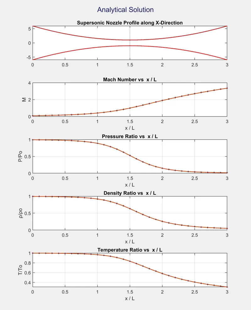
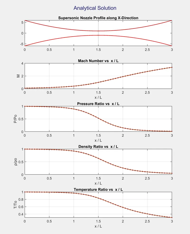
1. Characteristics Plot of Flow-Field Variables across the Nozzle at different Nodes along the X-Direction For the Analytical Solution.
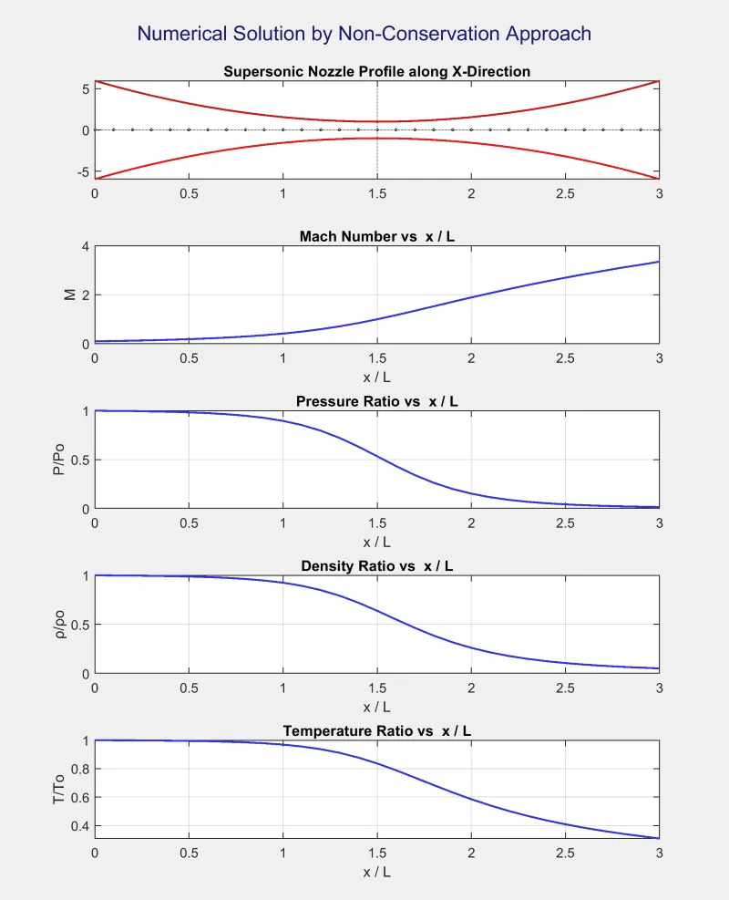
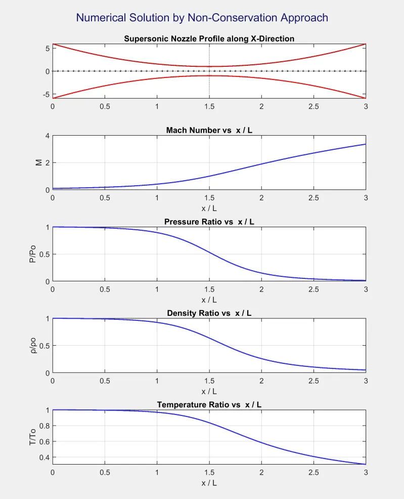
2. Characteristics Plot of Flow Variables across Nozzle at different Nodes along the X-Direction For the Non-Conservation Method Solution.
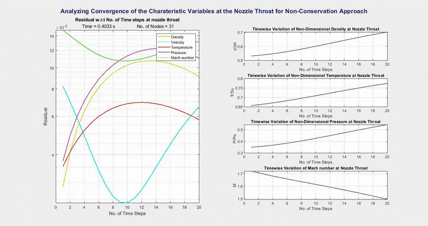
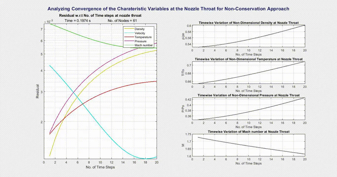
3. Observing Convergence at throat for Non-Conservation solution
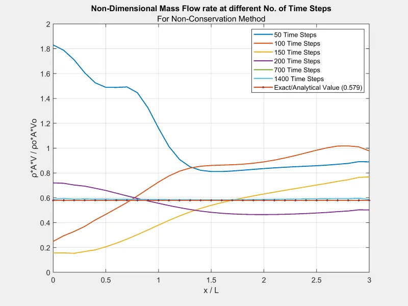
4. Mass Flow rate at Different No. of Time Steps For Non-Conservation Method
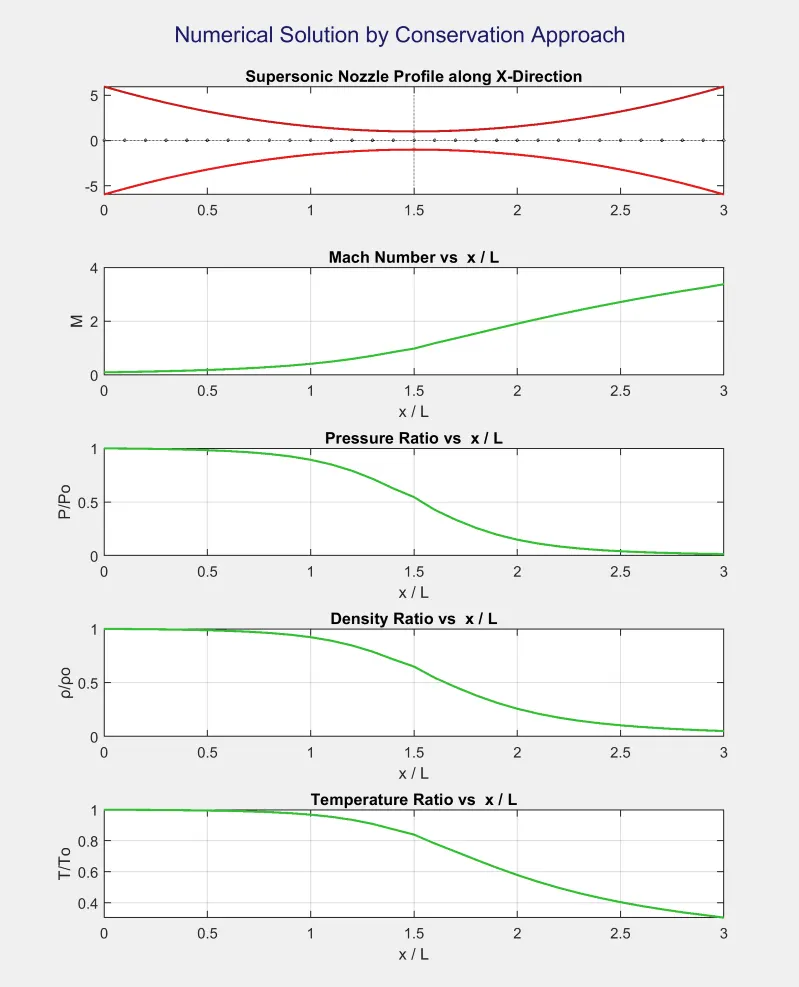
5. Characteristics Plot of Flow-Field Variables across the Nozzle at different Nodes along the X-Direction For the Conservation Method Solution.
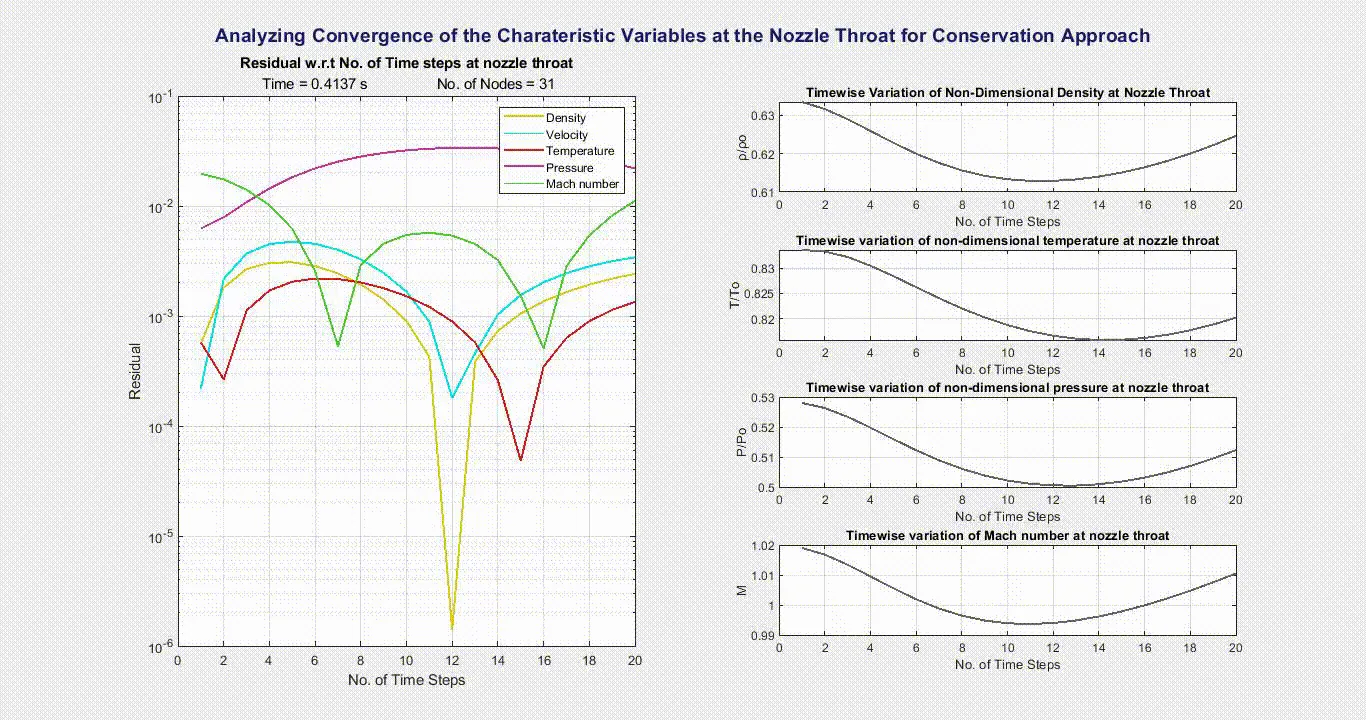
6. Observing Convergence at throat for Conservation solution
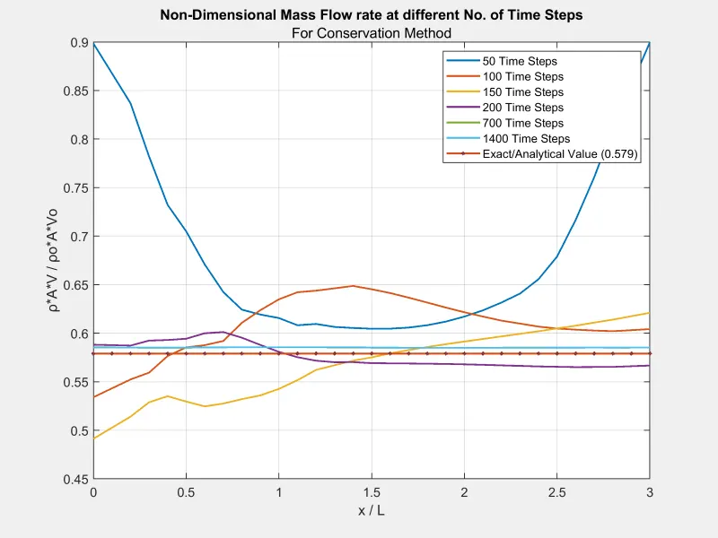
7. Mass Flow rate at Different No. of Time Steps For Conservation Method
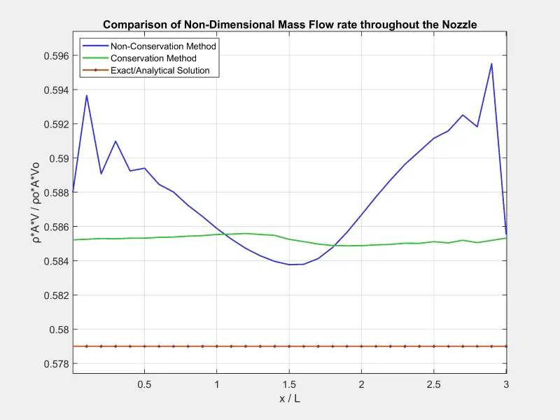
8. Comparison of Steady solution Non-Dimensional Mass Flow Rate from the different methods
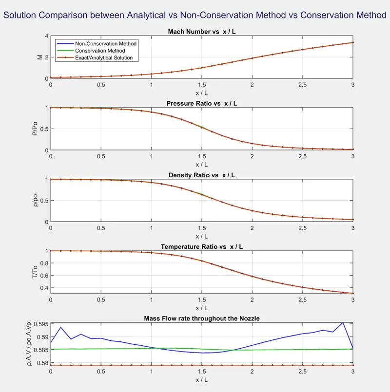
9. Comparison of Flow-Flowfield varlables plots between Analytical vs Non-Conservation Method vs Conservation Method
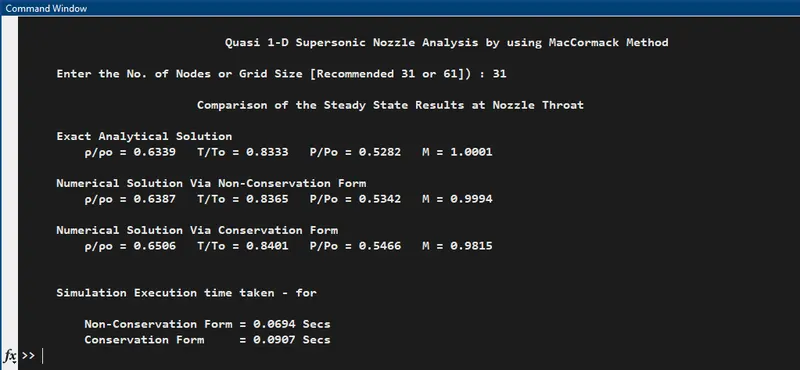
10. Checking difference in Values of the variables, by comparing values at the Nozzle Throat
- RESULTS AND OUTPUTS FOR THE ANALYSIS WITH - 61 NODES
1. Characteristics Plot of Flow-Field Variables across the Nozzle at different Nodes along the X-Direction For the Analytical Solution.
2. Characteristics Plot of Flow Variables across Nozzle at different Nodes along the X-Direction for the Non-Conservation Method Solution.
3. Observing Convergence at throat for Non-Conservation solution
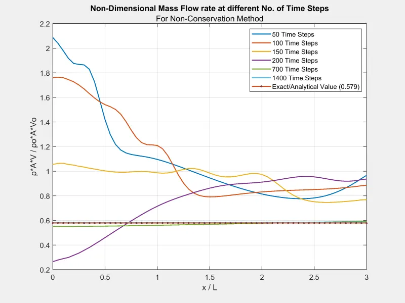
4. Mass Flow rate at Different No. of Time Steps For Non-Conservation Method
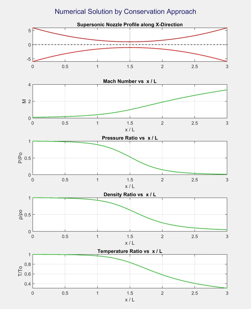
5. Characteristics Plot of Flow-Field Variables across the Nozzle at different Nodes along the X-Direction For the Conservation Method Solution.
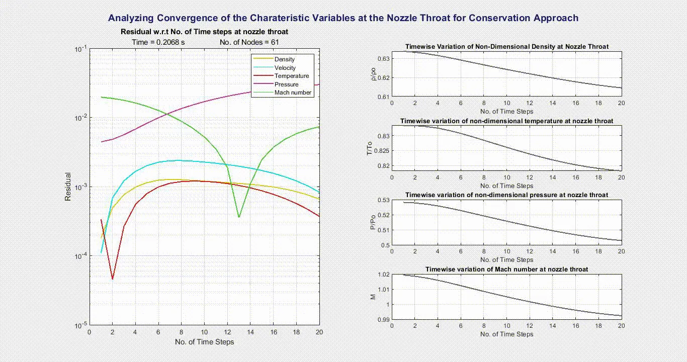
6. Observing Convergence at throat for Conservation solution
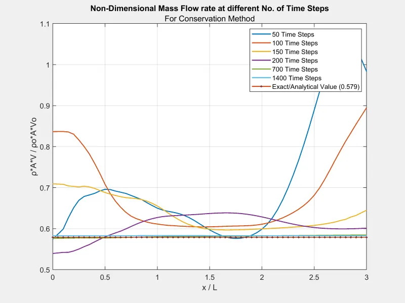
7. Mass Flow rate at Different No. of Time Steps For Conservation Method
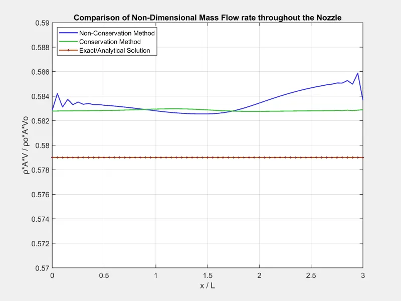
8. Comparison of Steady solution Non-Dimensional Mass Flow Rate from the different methods
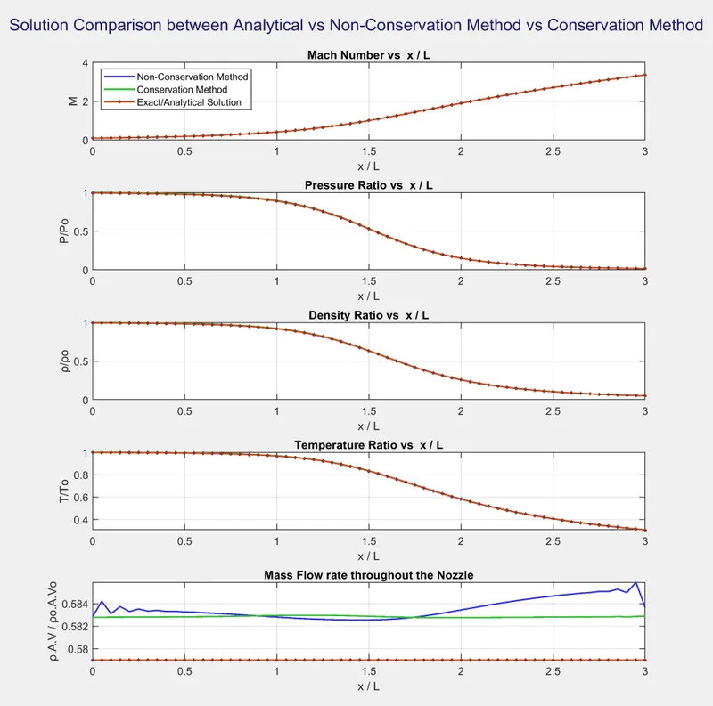
9. Comparison of Flow-Flowfield varlables plots between Analytical vs Non-Conservation Method vs Conservation Method
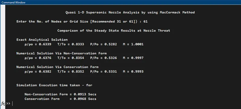
10. Checking difference in Values of the variables, by comparing values at the Nozzle Throat
RESULTS AND INFERENCE -
- Following is the sum up of the results we got after the simulation. (The table compares the values of the flow variables at the Nozzle Throat)
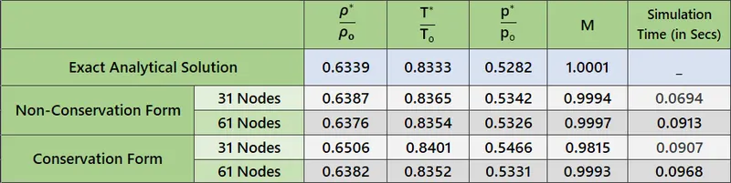
- Inorder for the grid independency test, we ran the simulation 2 times first with 31 Grid Points and second with 61 Grid Points. We can see the from the results that for the 61 points, we have just slightly more accurate solution. However the difference between the accuracy of 31 and 61 points is not much drastic. Raising even more the no. of grid points will give more accurate values but it will cost much high computional power and computation time. Therefore, a optimum simulation is the one which gives the reliable results in less cost and time.
- From the Residual plots (from plot 3 and 6), we can see the for the early part of Time-Step (Upto 600 steps) the residuals of Conservation methods were drasticaly dropping and converging compared to the Non-Conservation form. But after that for the next part of time-stepping the rate of residual getting smaller decreases compared to the non-conservation form.
- From the Mass-Flow Rate Plot, the Plots 4 and 7, we can see that at the 700th Time Step the Mass-flow rate values from conservation form are much closer to the analytical values compared to the Mass-Flow rate value of Non-Conservation Form at the 700th timestep. Also, Coservation form is more smoother and stable. This we can also see in the plot 8, the final steadty-state values of the conservation form are very smooth, while for the Non-Conservation form we can see the small peaks near to the boundaries.
- Coming to the conclusion, as per the plots and outputs,
- The Non-Conservation Mehtod Converges faster than the Conservation form.
- The Conservation Approach, give more accurate, smoother and stable values across the Nozzle, compared to the Non-Conservation.
- However, due to complexity in conservation form due to more mathematical term, it takes more computation time.
REFERENCES -
- John D. Anderson, Computational Fluid Dynamics : The Basics with Applications
- ME 702 - Computational Fluid Dynamics - Video Lesson 14 - YouTube
- http://www.thevisualroom.com/multi_step_methods.html#maccormack-method