Deriving 4th order approximation of a 2nd order derivative using Taylor Table method (ITCFDUML&OF/Challenge/Week3.5)
OBJECTIVE : To write a program to calculate 4rth order approximation for the 2nd order derivative of a function, from - Forward skewed, backward skewed and Central differencing.
- To derive the equations for the 4rth order appx. for forward skewed, backward skewed and central differencing using taylor table method.
- Calulating the analytical solution of 2nd order derivative of the function `f(x) = exp(x)*cos(x)`
- Estimating the solution from the derived equations of fourth order approximation, and compare accuracy between forward skewed, backward and central differencing by plotting the graphs.
THEORY :
The function, `f(x) = exp(x)*cos(x)`
considering at , `x = pi/3`
Analytical derivative - `f'(x) = exp(x)*cos(x)-exp(x)*sin(x)`
`f''(x) = -2*exp(x)*sin(x)`
Numerical Solution -
In this, we are doing 4rth order approximation for the second order derivative of the above function, considering for range of step size dx = [`pi/40 , pi/4000 , 200`].
4rth order appx. for 2nd derivative by -
- Forward Skewed Differencing
- Backward Skewed Differencing
- Central Differencing
Now finding the no. of points to be considered for the accuracy of the differencing.
So, for Forward & Backard schemes should satisfy, : P = N - Q
and for central differencing : P = N - Q + 1
Where, P = Order of accuracy
N = Number of nodes in the stencil
Q = Order of derivative
Therefore, For Forward and Backward Skewed, N = P + Q = 4 + 2
N = 6
and for central differencing, N = P + Q - 1 = 4 + 2 - 1
N = 5
Now Deriving the Equations for the for the 4rth Order Approxmation of 2nd Order Derivative using Taylor Table Method -
1. Forward Skewed Differencing
Here, N = 6.
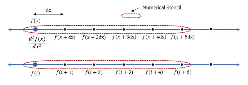
The equation can be written as,
`f''(x) = a.f(i) + b.f(i+1) + c.f(i+2) + d.f(i+3) + e.f(i+4) + g.f(i+5)`
Therefore applying Taylor Table Method,
| `f(x)` | `f'(x)`.dx | `f''(x)`.`(`d`x)^2` | `f'''(x)`.`(`d`x)^3` | `f''''(x)`.`(`d`x)^4` | `f'''''(x)`.`(`d`x)^5` | |
| `a.f(i)` | `a` | 0 | 0 | 0 | 0 | 0 |
| `b.f(i+1)` | `b` | `b` | `b/2` | `(b)/6` | `(b)/24` | `(b)/120` |
| `c.f(i+2)` | `c` | `2c` | `(4c)/2` | `(8c)/6` | `(16c)/24` | `(32c)/120` |
| `d.f(i+3)` | `d` | `3d` | `(9d)/2` | `(27d)/6` | `(81d)/24` | `(243d)/120` |
| `e.f(i+4)` | `e` | `4e` | `(16e)/2` | `(64e)/6` | `(256e)/24` | `(1024e)/120` |
| `g.f(i+5)` | `g` | `5g` | `(25g)/2` | `(125g)/6` | `(625g)/24` | `(3125g)/120` |
| `sum =` `(d^2f(x))/(dx^2)` | 0 | 0 | 1 | 0 | 0 | 0 |
Deducing into Linear Algebra -
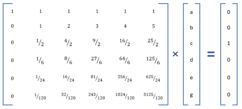
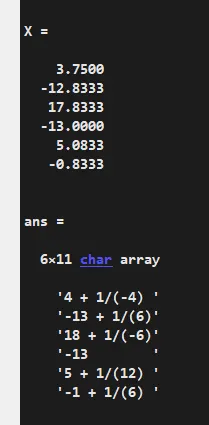
Using MATLAB to evaluate, we get,
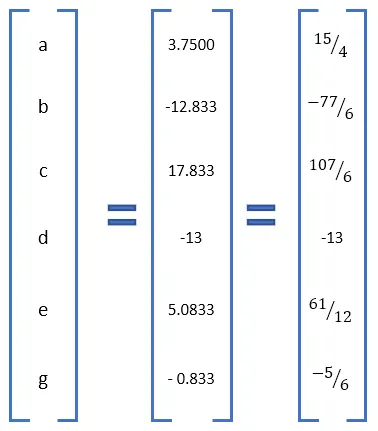
Therefore the Equation for the 4rth order appx. of 2nd order derivative with Forward skewed Differencing is -
`f''(x) = (3.7500).f(i) + (-12.833).f(i+1) + (17.833).f(i+2) + (-13).f(i+3) + (5.0833).f(i+4) + (- 0.833).f(i+5)`
or
`(d^2f(x))/(dx^2) = (45.f(i) - 154.f(i+1) + 214.f(i+2) - 156.f(i+3) + 61.f(i+4) - 10.f(i+5))/(12*dx)`
or
`(d^2f(x))/(dx^2) = (45.f(x) - 154.f(x+1dx) + 214.f(x+2dx) - 156.f(x+3dx) + 61.f(x+4dx) - 10.f(x+5dx))/(12*dx)`
-----------------------------------------------------------------------------------------------------------------------------------------------------
2. Backward Skewed Differencing
Here, N = 6.
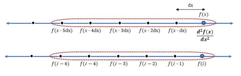
The equation can be written as,
`f''(x) = a.f(i) + b.f(i-1) + c.f(i-2) + d.f(i-3) + e.f(i-4) + g.f(i-5)`
Therefore applying Taylor Table Method,
| `f(x)` | `f'(x)`.dx | `f''(x)`.`(`d`x)^2` | `f'''(x)`.`(`d`x)^3` | `f''''(x)`.`(`d`x)^4` | `f'''''(x)`.`(`d`x)^5` | |
| `a.f(i)` | `a` | 0 | 0 | 0 | 0 | 0 |
| `b.f(i-1)` | `b` | `-b` | `b/2` | `(-b)/6` | `(b)/24` | `(-b)/120` |
| `c.f(i-2)` | `c` | `-2c` | `(4c)/2` | `(-8c)/6` | `(16c)/24` | `(-32c)/120` |
| `d.f(i-3)` | `d` | `-3d` | `(9d)/2` | `(-27d)/6` | `(81d)/24` | `(-243d)/120` |
| `e.f(i-4)` | `e` | `-4e` | `(16e)/2` | `(-64e)/6` | `(256e)/24` | `(-1024e)/120` |
| `g.f(i-5)` | `g` | `-5g` | `(25g)/2` | `(-125g)/6` | `(625g)/24` | `(-3125g)/120` |
| `sum =` `(d^2f(x))/(dx^2)` | 0 | 0 | 1 | 0 | 0 | 0 |
Deducing into Linear Algebra -
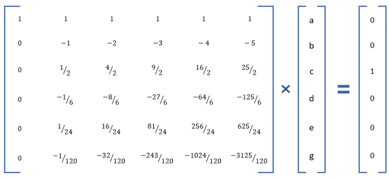
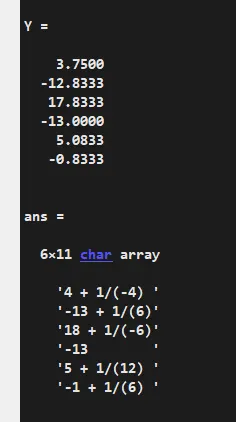
Using MATLAB to evaluate, we get,
Therefore the Equation for the 4rth order appx. of 2nd order derivative with Backward skewed Differencing is -
`f''(x) = (3.7500).f(i) + (-12.833).f(i-1) + (17.833).f(i-2) + (-13).f(i-3) + (5.0833).f(i-4) + (- 0.833).f(i-5)`
or
`(d^2f(x))/(dx^2) = (45.f(i) - 154.f(i-1) + 214.f(i-2) - 156.f(i-3) + 61.f(i-4) - 10.f(i-5))/(12*dx)`
or
`(d^2f(x))/(dx^2) = (45.f(x) - 154.f(x-1dx) + 214.f(x-2dx) - 156.f(x-3dx) + 61.f(x-4dx) - 10.f(x-5dx))/(12*dx)`
----------------------------------------------------------------------------------------------------------------------------------------------------
3. Central Differencing
Here, N = 5.
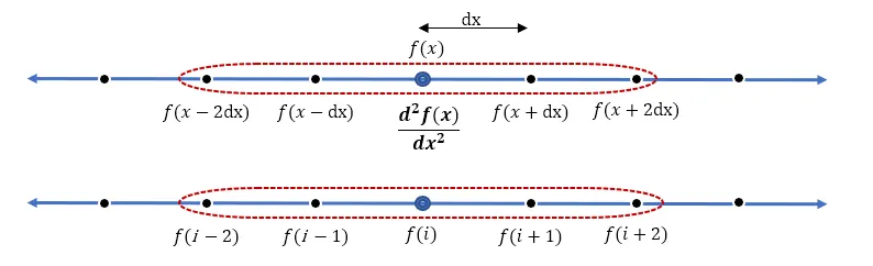
The equation can be written as,
`f''(x) = a.f(i-2) + b.f(i-1) + c.f(i) + d.f(i+1) + e.f(i+2) `
Therefore applying Taylor Table Method,
| `f(x)` | `f'(x)`.dx | `f''(x)`.`(`d`x)^2` | `f'''(x)`.`(`d`x)^3` | `f''''(x)`.`(`d`x)^4` | `f'''''(x)`.`(`d`x)^5` | |
| `a.f(i-2)` | `a` | `-2a` | `(4a)/2` | `(-8a)/6` | `(16a)/24` | `(-32a)/120` |
| `b.f(i-1)` | `b` | `-b` | `b/2` | `(-b)/6` | `(b)/24` | `(-b)/120` |
| `c.f(i)` | `c` | `0` | `0` | `0` | `0` | `0` |
| `d.f(i+1)` | `d` | `3d` | `d/2` | `(d)/6` | `(d)/24` | `(d)/120` |
| `e.f(i+2)` | `e` | `2a` | `(4a)/2` | `(8a)/6` | `(16a)/24` | `(32a)/120` |
| `sum =` `(d^2f(x))/(dx^2)` | 0 | 0 | 1 | 0 | 0 | -- |
Deducing into Linear Algebra -
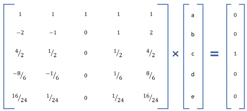
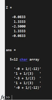
Using MATLAB to evaluate, we get,
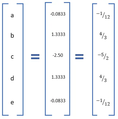
Therefore the Equation for the 4rth order appx. of 2nd order derivative with Central Differencing is -
`f''(x) = (-0.0833).f(i-2) + (1.333).f(i-1) + (-2.5).f(i) + (1.333).f(i+1) + (-0.0833).f(i+2) `
or
`(d^2f(x))/(dx^2) = (- 1.f(i-2) + 16.f(i-1) - 30.f(i) + 16.f(i+1) - 1.f(i+2))/(12*dx)`
or
`(d^2f(x))/(dx^2) = (- 1.f(x-2dx) + 16.f(x-dx) - 30.f(x) + 16.f(x+dx) - 1.f(x+2dx))/(12*dx)`
------------------------------------------------------------------------------------------------------------------------------------------
PROGRAM :
% 4rth order Approximation of 2nd order derivate

clear all;
close all;
clc;


% Function-   f(x) = exp(x)*cos(x)
%            f'(x) = exp(x)*cos(x)-exp(x)*sin(x)
%           f''(x) = -2*exp(x)*sin(x)

% Analytical Solution
x = pi/5;

anal_dev = -2*exp(x)*sin(x);

dx = linspace(pi/40,pi/400,200);


%------------- Forward skewed ----------------

A = [1 1 1 1 1 1; 0 1 2 3 4 5; 0 1/2 2 9/2 16/2 25/2; 0 1/6 8/6 27/6 64/6 125/6; 0 1/24 16/24 81/24 256/24 625/24; 0 1/120 32/120 243/120 1024/120 3125/120 ];
B = [0; 0; 1; 0; 0; 0];

X = inv(A)*B
rat(X)

%-------------- Backward skewed --------------

A = [1 1 1 1 1 1; 0 -1 -2 -3 -4 -5; 0 1/2 2 9/2 16/2 25/2; 0 -1/6 -8/6 -27/6 -64/6 -125/6; 0 1/24 16/24 81/24 256/24 625/24; 0 -1/120 -32/120 -243/120 -1024/120 -3125/120 ];
B = [0; 0; 1; 0; 0; 0];

Y = inv(A)*B
rat(Y)

% --------------- Central Differencing --------------
A = [ 1 1 1 1 1; -2 -1 0 1 2; 2 1/2 0 1/2 2; -8/6 -1/6 0 1/6 8/6; 16/24 1/24 0 1/24 16/24];
B = [0; 0; 1; 0; 0];

Z = inv(A)*B
rat(Z)

%--------------------------------------------------------------------------------------------

for i = 1:length(dx)

    forward_diff(i)  = ( (X(1)*exp(x)*cos(x)) + (X(2)*exp(x+dx(i))*cos(x+dx(i))) + (X(3)*exp(x+2*dx(i))*cos(x+2*dx(i))) + ...
                         + (X(4)*exp(x+3*dx(i))*cos(x+3*dx(i))) + (X(5)*exp(x+4*dx(i))*cos(x+4*dx(i))) + (X(6)*exp(x+5*dx(i))*cos(x+5*dx(i))) )/(dx(i)^2) ;

    backward_diff(i) = ( (Y(1)*exp(x)*cos(x)) + (Y(2)*exp(x-dx(i))*cos(x-dx(i))) + (Y(3)*exp(x-2*dx(i))*cos(x-2*dx(i))) + ...
                         + (Y(4)*exp(x-3*dx(i))*cos(x-3*dx(i))) + (Y(5)*exp(x-4*dx(i))*cos(x-4*dx(i))) + (Y(6)*exp(x-5*dx(i))*cos(x-5*dx(i))) )/(dx(i)^2) ;

    central_diff(i)  = ( (Z(1)*exp(x-2*dx(i))*cos(x-2*dx(i))) + (Z(2)*exp(x-dx(i))*cos(x-dx(i))) + (Z(3)*exp(x)*cos(x)) + ...
                         + (Z(4)*exp(x+dx(i))*cos(x+dx(i))) + (Z(5)*exp(x+2*dx(i))*cos(x+2*dx(i))) )/(dx(i)^2)  ;


    err_fd(i) = abs(forward_diff(i) - anal_dev);
    err_bd(i) = abs(backward_diff(i) - anal_dev);
    err_cd(i) = abs(central_diff(i) - anal_dev);

end


figure(1)
plot(dx,err_fd,'color','b','linewidth',1.5);
hold on;    grid on;
plot(dx,err_bd,'color','g','linewidth',1.5);
plot(dx,err_cd,'color','r','linewidth',1.5);
xlabel('dx');   ylabel(' Error');
legend('Error Forward Differencing','Error Backward Differencing','Error Central Differencing','Location','northwest');

figure(2)
loglog(dx,err_fd,'color','b','linewidth',1.5);
hold on;    grid on;
loglog(dx,err_bd,'color','g','linewidth',1.5);
loglog(dx,err_cd,'color','r','linewidth',1.5);
xlabel('dx');   ylabel(' Error');
legend('Error Forward Differencing','Error Backward Differencing','Error Central Differencing','Location','northwest');
OUTPUT :
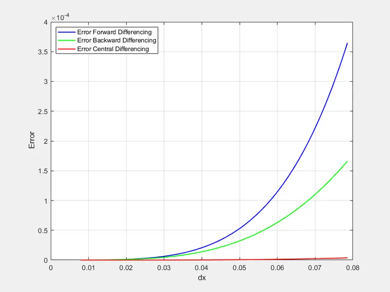
Plot 1 -
Plot 2 -
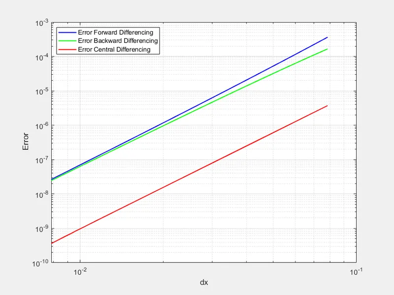
RESULT :
From the Output plot we can see that for the 4rth order approximation, the central differencing is more accurate i.e. having less error than the backward skewed and forward skewed differencing.
The Central Differencing is mostly used in middle region of the grid space. Since, its is symmetric and requires same no. of nodes from both direction. And therefore, for the region closer to the boundaries the forward & backward skewed Differencing is used.