Week 7 - Simulation of a 1D Super-sonic nozzle flow simulation using Macormack Method
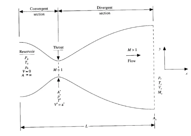
In this problem isentropic flow through a convergent-Divergent nozzle is shown in the figure below. The flow at the inlet to the nozzle comes from a reservoir where the pressure and temperature are denoted by p0 , and To, respectively. The cross-sectional area of the reservoir is large , and hence the velocity is very small ( V --> O). Thus, Po and T0 are the stagnation values, or total pressure and total temperature, respectively. The flow expands Isentropically to supersonic speeds at the nozzle exit, where the exit pressure, temperature, velocity, and Mach number are denoted by Pe, Te, Ve, and Me, respectlvely. The flow is locally subsonic in the convergent section of the nozzle, some at the throat (minimum area), and supersonic at the divergent section. The sonic flow (M = 1) at the throat means that the local velocity at this location is equal to the local speed of sound.
The problem can be solved by two methods:
1. Non-Conservative Form
Governing Equations
The governing equations employed in solving the equations is given by
Continuity: `rho1*A1*V1 = rho2*A2*V2`
Momentum: `rho1*A1 + rho1*V1^2*A1 + int p dA = p2*A2 + rho2*V2^2*A2`
Energy: `h1 + V1^2//2 = h2 + V2^2//2`
These equations can be further extended in non conservative form as-
Continuity Equation: `delrho//delt = -rho**delV//delx - rho*V*del(lnA)//delx -V*delrho//delx`
`delV//delt = -V*delV//delx - (1/gamma)*(delT//delx+T/rho *delp//delx)`
Energy Equation : `delT//delt = -V*delT//delx -(gamma-1)T(delV//delx + Vdel(lnA)//delx)`
Further the problem is solved by three steps:
1.Mesh
2. Discretize
3. Solve
a.)Initial condition
b.) Boundary condition
1. As the mesh is made from the number of points at which we want output and the outer points are defined. The initial point is defined as fixed and the last step is governed by previous ones. And the problem is solved for inner nodes.
2. Discretization is done by Mc Cormack technique.
This is done in explicit method
Initial Condition: predictor step: In this step the space terms are written as forward differenced. `deltaf//deltat_p`
Solution Update: `f^* = f(old) + delf//delt * Deltat`
Corrector step: In this step the space terms are written as Backward differenced. `delf^*//delt_c`
`delf//delt_(avg) = 0.5*(delf//delt_p + delf^*//delt_c)`
`f^(2nd time step) = f(old) + delf//delt_(avg) *Deltat`
The values of starting conditions are
`rho = 1 - 0.3146*X`
`T = 1. 0.2314*X`
`V = (0.1 + 1.09*X)T^(1/2)`
The changing area is calculated as
`A = 1 + 2.2(x-1.5)^2` `0<=x<=3`
The matlab code is
function[rho,t,mach,m,rho_t,p_r,t_t,pr_r_t,mach_t]=non_conservative_update(x,dx,gamma,a,nt)

%NON CONSERVATIVE FORM
%calculate initial profiles
rho = 1 - 0.3146*x;
t = 1-0.2314*x; %t = temperature
v = (0.1 + 1.09*x).*t.^0.5 ;


%Time steps
nt = 1000;
dt = 0.01;
n=31

%Outer time loop
for k = 1:nt

    rho_old = rho;
    v_old = v;
    t_old = t;

    %Predictor time step
    for j=2:n-1
        %drho_dt_p = -rho(j)*((v(j+1)-v(j))/dx) - rho(j)*v(j)*((log(a(j+1))-log(a(j)))/dx) - v(j)*((rho(j+1)-rho(j))/dx);

        %alternate form
        dvdx = (v(j+1)-v(j))/dx;
        drhodx = (rho(j+1)-rho(j))/dx;
        dtdx = (t(j+1)-t(j))/dx;
        dloga_dx = (log(a(j+1))-log(a(j)))/dx;

        %Continuity equation
        drho_dt_p(j) = -rho(j)*dvdx -rho(j)*v(j)*dloga_dx -v(j)*drhodx;

        %Momentum equation
        dv_dt_p(j) = -v(j)*dvdx-(1/gamma)*(dtdx + (t(j)/rho(j))*drhodx);

        %Energy Equation
        dt_dt_p(j) = -v(j)*dtdx -(gamma - 1)*t(j)*(dvdx+v(j)*dloga_dx);

        %Solution Update
        rho(j) = rho(j) + drho_dt_p(j)*dt;
        v(j) = v(j) + dv_dt_p(j)*dt;
        t(j) = t(j) + dt_dt_p(j)*dt;

    end

    %corrector time step
    for j=2:n-1
        %drho_dt_p = -rho(j)*((v(j)-v(j-1))/dx) - rho(j)*v(j)*((log(a(j))-log(a(j-1)))/dx) - v(j)*((rho(j)-rho(j-1))/dx);

        %alternate form
        dvdx = (v(j)-v(j-1))/dx;
        drhodx = (rho(j)-rho(j-1))/dx;
        dtdx = (t(j)-t(j-1))/dx;
        dloga_dx = (log(a(j))-log(a(j-1)))/dx;

        %Continuity equation
        drho_dt_c(j) = -rho(j)*dvdx -rho(j)*v(j)*dloga_dx -v(j)*drhodx;

        %Momentum equation
        dv_dt_c(j) = -v(j)*dvdx-(1/gamma)*(dtdx + (t(j)/rho(j))*drhodx);

        %Energy Equation
        dt_dt_c(j) = -v(j)*dtdx -(gamma - 1)*t(j)*(dvdx+v(j)*dloga_dx);

    end

    %COmputing avg. time step

    dv_dt = 0.5*(dv_dt_p + dv_dt_c);
    drho_dt = 0.5*(drho_dt_p + drho_dt_c);
    dt_dt = 0.5*(dt_dt_p + dt_dt_c);

    for i=2:n-1

        %Final time update
        rho(i) = rho_old(i) + drho_dt(i)*dt;
        v(i) = v_old(i)+ dv_dt(i)*dt;
        t(i) = t_old(i) + dt_dt(i)*dt;


    end

    %Applying boundary conditions
    %Inlet
    v(1) = 2*v(2) - v(3);

    %outlet
    v(n) = 2*v(n-1) - v(n-2);
    rho(n) = 2*rho(n-1) - rho(n-2);
    t(n) = 2*t(n-1) - t(n-2);

    %MAss flow rate
    m = rho.*v.*a;
    %Mach no.
    mach = v./(t.^0.5);
    %pressure ratio
    p_r = rho.*t;

    %values at throat
    rho_t(k) = rho(16);
    t_t(k) = t(16);
    pr_r_t(k) = p_r(16);
    mach_t(k) = mach(16);


    figure(4)
    if k==50;
        plot(x,m)
        xlabel('Non Dimensional mass flow rate')
        ylabel('Non Dimensional length')
        title('Variation of mass flow rate at different time steps in Non-Conservative form')
        hold on
    elseif k == 100
        plot(x,m)
        hold on
    elseif k == 200
        plot(x,m)
        hold on
    elseif k == 400
        plot(x,m)
        hold on
    elseif k == 800
        plot(x,m)
        hold on
    elseif k == 900
        plot(x,m)
        hold on
    elseif k == 1000
        plot(x,m)
        hold on
    elseif k == 1200
        plot(x,m)
        hold on
    elseif k == 1400
        plot(x,m)
        legend('50th Timestep','100th Timestep','200th Timestep','400th Timestep','800th Timestep','900th Timestep','1000th Timestep','12000th Timestep','1400th Timestep')
    end

end
end
2. Conservative Form
Continuity Equation: `delta(rhoA)//deltat = - delta(AV)//deltax`
Momentum Equation: `delta(rhoAV)//deltat + delta(rhoAV^2 + (1/gamma)rhoA)//deltax = (1/gamma)pdeltaA//deltax`
Energy Equation: `delta(rho(e/(gamma-1)+(gamma/2)V^2)A)//deltat + delta(rho(e/(gamma-1)+(gamma/2)V^2)VA+rhoAV)//deltax`
where e is Internal energy
For the ease of writing code we converted the forms,
`U1 = rhoA`
`U2 = rhoAV`
`U3 = rho(e/(gamma-1)+(gamma/2)V^2)A`
`F1= rhoAV`
`F2 = rhoAV^2`
`F3 = rho(e/(gamma-1)+(gamma/2)V^2)VA+rhoAV`
`J2 = (1/gamma)p*deltaA//deltax`
The final equations can be written as
Continuity Equation: `delU1//delt = -delF1//delx`
Momentum Equation: `delU2//delt = -delF2//delx + J2`
Energy Equation: `delU3//delt = -delF3//delx`
Boundary Conditions:
for `0<=x<=0.5` --> `{rho=1 &T=1}`
for `0.5<=x<=1.5` --> `{rho = 1-0.366(x-0.5) &T=1-0.167(x-0.5)}`
for `1.5<=x<=3` --> `{rho = 0.634-0.3879(x-1.5)&T=0.833-0.3507(x-1.5)}`
The matlab code is
function[rho_c,t_c,mach_c,m_c,p_c,rho_tc,t_tc,pr_r_tc,mach_tc]=conservative_update(x,dx,gamma,a,nt)

%CONSERVATIVE FORM
n=31
%Initial conditions
for i=1:n
    if x(i)>=0 && x(i)<0.5
        rho_c(i) = 1;
        t_c(i) = 1;
    elseif x(i)>=0.5 && x(i)<1.5
        rho_c(i)= 1-0.366*(x(i)-0.5);
        t_c(i) = 1-0.167*(x(i)-0.5);
    elseif x(i)>=1.5 && x(i)<=3.5
        rho_c(i)= 0.634-0.3879*(x(i)-1.5);
        t_c(i) = 0.833-0.3507*(x(i)-1.5);
    end
end


v_c = 0.59./(rho_c.*a);
dt = 0.0267;

U1 = rho_c.*a;
U2 = rho_c.*a.*v_c;
U3 = U1.*((t_c./(gamma - 1)) + ((gamma./2).*v_c.^2));


%Time steps
nt = 1400;


%Outer time loop
for k = 1:nt
    U1_old = U1;
    U2_old = U2;
    U3_old = U3;


    F1 = U2;
   %F2 = ((U2.^2)./U1) + (gamma-1/gamma)*U3-(gamma/2)*((U2.^2)./U1); ERROR
    F2 = ((U2.^2)./U1) + ((gamma-1)/gamma)*(U3-(gamma/2)*((U2.^2)./U1));
    F3 = (gamma.*U2.*U3)./U1  - ((gamma*(gamma-1)*0.5)*(U2.^3./U1.^2));


    for j=2:n-1
        %predictor step
        J(j) = (1/gamma)*rho_c(j).*t_c(j).*((a(j+1)-a(j))/dx);

        du1_dt_p(j) = -((F1(j+1) - F1(j))/dx);
        du2_dt_p(j) = -((F2(j+1) - F2(j))/dx) + J(j);
        du3_dt_p(j) = -((F3(j+1) - F3(j))/dx);

        %Solution Update
        U1(j) = U1(j) + (du1_dt_p(j)*dt);
        U2(j) = U2(j) + (du2_dt_p(j)*dt);
        U3(j) = U3(j) + (du3_dt_p(j)*dt);

    end
    rho_c = U1./a;
    v_c = U2./U1;
    t_c = (gamma-1)*((U3./U1)-(gamma/2)*v_c.^2);
    p_c = rho_c.*t_c;
    F1 = U2;
   % F2 = ((U2.^2)./U1) + ((gamma-1/gamma)*(U3-(gamma/2)*((U2.^2)./U1)));
   % ERROR
    F2 = ((U2.^2)./U1) + ((gamma-1)/gamma)*(U3-(gamma/2)*((U2.^2)./U1));
    F3 = (gamma.*U2.*U3)./U1  - ((gamma*(gamma-1)*0.5)*(U2.^3./U1.^2));

    for j =2:n-1
        J(j) = (1/gamma)*rho_c(j).*t_c(j).*((a(j)-a(j-1))/dx);
        %corrector step
        du1_dt_c(j) = -((F1(j) - F1(j-1))/dx);
        du2_dt_c(j) = -((F2(j) - F2(j-1))/dx) + J(j);
        du3_dt_c(j) = -((F3(j) - F3(j-1))/dx);

    end

    du1_dt = 0.5*(du1_dt_p + du1_dt_c);
    du2_dt = 0.5*(du2_dt_p + du2_dt_c);
    du3_dt = 0.5*(du3_dt_p + du3_dt_c);
    for m=2:n-1

        U1(m) = U1_old(m) + (du1_dt(m)*dt);
        U2(m) = U2_old(m) + (du2_dt(m)*dt);
        U3(m) = U3_old(m) + (du3_dt(m)*dt);
    end


    % updation of properties
    v_c = U2./U1;
    t_c = (gamma-1)*((U3./U1)-(gamma/2)*v_c.^2);
    rho_c = U1./a;
    p_c = rho_c.*t_c;
    m_c = rho_c.*a.*v_c;
    mach_c = v_c./(t_c.^0.5);

    U1(1) = rho_c(1)*a(1);
    U2(1) = 2*U2(2)-U2(3);
    U3(1) = ((t_c(1)/(gamma-1))+(gamma*0.5*(v_c(1)^2)))*U1(1);
    U1(n) = 2*U1(n-1)-U1(n-2);
    U2(n) = 2*U2(n-1)-U2(n-2);
    U3(n) = 2*U3(n-1)-U3(n-2);

    %values at throat
    rho_tc(k) = rho_c(16);
    t_tc(k) = t_c(16);
    pr_r_tc(k) = p_c(16);
    mach_tc(k) = mach_c(16);


    figure(2)
    if k==50;
        plot(x,m_c)
        hold on
    elseif k == 100
        plot(x,m_c)
        hold on
    elseif k == 200
        plot(x,m_c)
        hold on
    elseif k == 400
        plot(x,m_c)
        hold on
    elseif k == 800
        plot(x,m_c)
        hold on
    elseif k == 900
        plot(x,m_c)
        hold on
    elseif k == 1000
        plot(x,m_c)
        hold on
    elseif k == 1200
        plot(x,m_c)
        hold on
    elseif k == 1400
        plot(x,m_c)
        xlabel('Non Dimensional mass flow rate')
        ylabel('Non Dimensional length')
        title('Variation of mass flow rate at different time steps in conservative form')
        legend('50th Timestep','100th Timestep','200th Timestep','400th Timestep','800th Timestep','900th Timestep','1000th Timestep','12000th Timestep','1400th Timestep')
    end
end
end
The final Matlab code to call out both of the functions and solving them is
The results obtained are discussed below-
clear all
close all
clc

n=31;
x = linspace(0,3,n);
dx = x(2) - x(1);
gamma = 1.4;
%area
a = 1+2.2*(x-1.5).^2;
nt =1400;
n=31;

[rho,t,mach,m,rho_t,p_r,t_t,pr_r_t,mach_t]=non_conservative_update(x,dx,gamma,a,nt)
[rho_c,t_c,mach_c,m_c,p_c,rho_tc,t_tc,pr_r_tc,mach_tc]=conservative_update(x,dx,gamma,a,nt)


%Conservative plots
figure(1)
subplot(4,1,1)
plot(x,rho_c)
grid minor
title('Steady state distribution of primitive variable of conserrvative form')
xlabel('Non Dimensional Length')
ylabel('Density')
subplot(4,1,2)
plot(x,t_c)
grid minor
xlabel('Non Dimensional Length')
ylabel('Temperature')
subplot(4,1,3)
plot(x,mach_c)
grid minor
xlabel('Non Dimensional Length')
ylabel('Mach Number')
subplot(4,1,4)
plot(x,p_c)
grid minor
xlabel('Non Dimensional Length')
ylabel('Pressure')

%PLots at throat section
 figure(3)
 subplot(4,1,1)
 plot(rho_tc)
 grid minor
 xlabel('Timestep')
 ylabel('density')
 title('Time wie variation of primitive vairables at throat for conservative form')
 subplot(4,1,2)
 plot(t_tc)
 grid minor
 xlabel('Timestep')
 ylabel('Temperature')
 subplot(4,1,3)
 plot(pr_r_tc)
 grid minor
 xlabel('Timestep')
 ylabel('Presuure')
 subplot(4,1,4)
 plot(mach_tc)
 grid minor
 xlabel('Timestep')
 ylabel('Mach no.')


 %Non-Conservative plots
figure(5)
subplot(4,1,1)
plot(x,rho)
grid minor
title('Steady state distribution of primitive variable of non-conserrvative form')
xlabel('Non Dimensional Length')
ylabel('Density')
subplot(4,1,2)
plot(x,t)
grid minor
xlabel('Non Dimensional Length')
ylabel('Temperature')
subplot(4,1,3)
plot(x,mach)
grid minor
xlabel('Non Dimensional Length')
ylabel('Mach Number')
subplot(4,1,4)
plot(x,p_r)
grid minor
xlabel('Non Dimensional Length')
ylabel('Pressure')


%PLots at throat section
 figure(6)
 subplot(4,1,1)
 plot(rho_t)
 grid minor
 xlabel('Timestep')
 ylabel('density')
 title('Time wie variation of primitive vairables at throat for non conservative form')
 subplot(4,1,2)
 plot(t_t)
 grid minor
 xlabel('Timestep')
 ylabel('Temperature')
 subplot(4,1,3)
 plot(pr_r_t)
 grid minor
 xlabel('Timestep')
 ylabel('Presuure')
 subplot(4,1,4)
 plot(mach_t)
 grid minor
 xlabel('Timestep')
 ylabel('Mach no.')


 %PLotting Mass flow rate
 figure(7)
 plot(x,m_c)
 hold on
 plot(x,m)
 xlabel('Length of Nozzle')
 ylabel('Mass flow rate')
 title('Comaparision of mass flow rate')
 legend('Conservative','Non-Conservative')
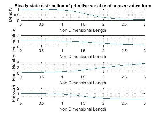
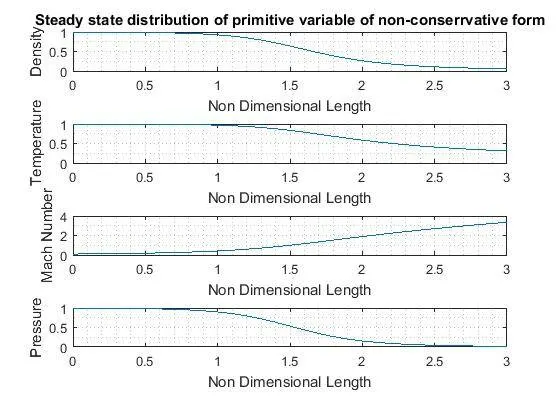
1. Steady State distribution of primitive variables
For conservative:
For non conservative:
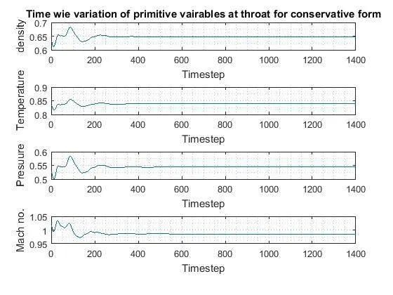
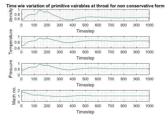
2. Time Wise variation of primitive variables at throat
For conservative:
For non conservative:
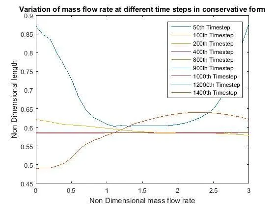
3. Mass Flow rate at different Time Steps
For Conservative:
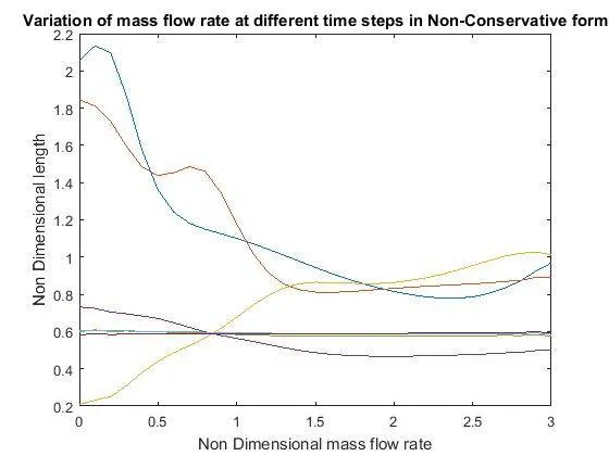
For Non-Conservative:
4. Comparision of Normalised Mass Flow rate in both forms:
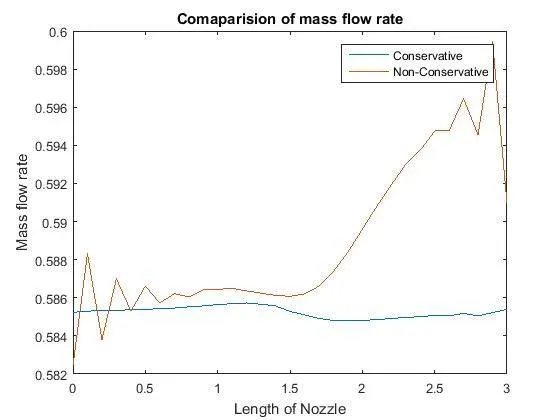
As from the above plot, it is clear that the stability of mass flow rate in conservative form is more as compared to Non-conservative Form. So, it can be concluded that there are more chances of getting some flashes in result in the form of error when non conservative form is taken into consideration.
Grid Dependency Test:
As in this test the simulation for both conservative an dnon conservative form is run at N=31 and 61 grid ponts, and the result is recorded below.
| `rho^'/rho_0` | `T^'/T_0` | `P^'/P_0` | M | |
|
Exact analytical solution |
0.634 | 0.833 | 0.528 | 1.000 |
|
31 Points Non Conservative |
0.639 | 0.836 | 0.534 | 0.999 |
|
31 Points Conservative |
0.629 | 0.858 | 0.595 | 0913 |
|
61 Points Non Conservative |
0.638 | 0.835 | 0.533 | 1.000 |
|
61 Points Conservative |
0.639 | 0.835 | 0.534 | 0.998 |
From the above table, It can be concluded that the solution converges to the exact solution when there are more number of grid points employed. Also further this can be inferred that the Conservative form form will give better results.
So the conservative approach with more number of grid points will give results NS equation when solved with minimum error.