Week 5: Prandtl Meyer Shock problem
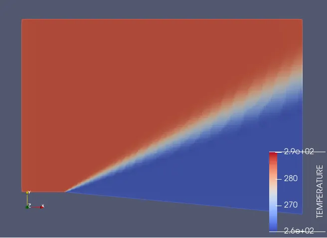
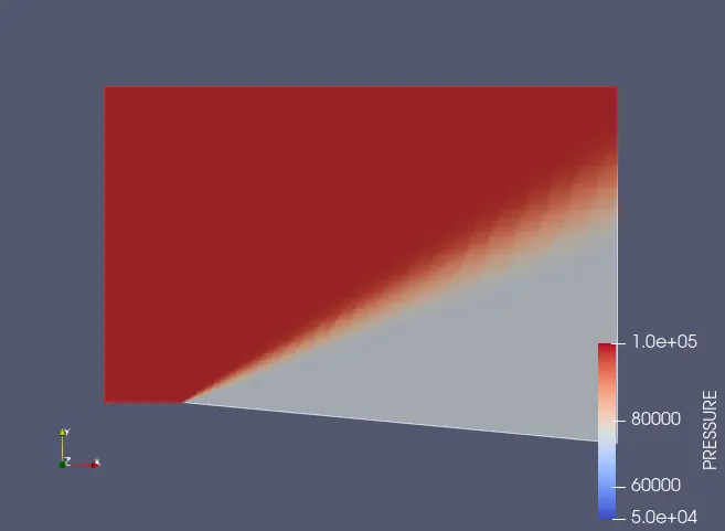
A centered, Prandtl-Meyer expansion wave is illustrated in Fig. below. Here, a supersonic flow is expanded around a sharp expansion comer. An expansion wave, made up of an infinite number of infinitely weak Mach waves, fans out from the comer, as shown in Fig. below. The leading edge of the expansion fan makes an angle μ1 with respect to the upstream flow direction, and the trailing edge of the wave makes an angle μ2 with respect to the downstream flow direction.
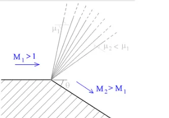
where M1 and M2 are the upstream and downstream Mach numbers, respectively. The flow through an expansion wave is isentropic. As the flow passes through the expansion wave, the Mach number increases and the pressure, temperature, and density decrease. The flow in front of the centered expansion wave is uniform at a Mach number M1 and is parallel to the wall in front of the wave. The flow behind the expansion wave is also uniform at a Mach number of M2 and is parallel to the wall behind the wave. Inside the wave itself, the flow properties change smoothly, and the streamlines are curved. The only exception to the above discussion is right at the comer itself; this is a singular point at which the streamline at the wall experiences a discontinuous change in direction and where the flow properties are discontinuous. This singularity has some impact on the numerical solution of the flow field, as you might suspect. Such matters will be addressed in a subsequent section.
Types of Boundary conditions:
Both ordinary and partial differential equations need boundary conditions to be solved. Different types of boundary conditions can be imposed on the boundary of the domain. The choice of the boundary condition is fundamental for the resolution of the computational problem: a bad imposition of b.c. may lead to the divergence of the solution or to the convergence to a wrong solution.
Dirichlet Boundary Condition
The Dirichlet boundary condition is a type of boundary condition named after Peter Gustav Lejeune Dirichlet. Dirichlet boundary condition is a type of boundary condition, where numerical value is given directly to boundary faces. It is also referred to as first-type boundary condition.
Examples include flow velocity of 5 m/s and temperature 20 °C.
Neumann Boundary Condition
The Neumann boundary condition is a type of boundary condition, named after Carl Neumann. When imposed on an ordinary (ODE) or a partial differential equation (PDE), it specifies the values that the derivative of a solution is going to take on the boundary of the domain. The gradient can be thought of as the rate of change. Conditions such as a free-slip condition and an adiabatic condition are examples of Neumann boundary conditions.
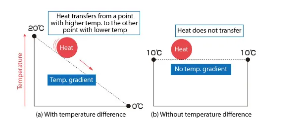
For example, consider an adiabatic condition as shown in figure. When the temperatures at two points are different, heat transfers from the point with higher temperature to the point with the lower temperature. An adiabatic condition means no heat is transferred. This is achieved by having the temperatures of the two points be the same. When the temperatures of the two points are the same, the temperature gradient (rate of change) is 0. Therefore, an adiabatic condition can be expressed by a Neumann boundary condition with a temperature gradient equal to 0.
Robin Boundary Condition
The Robin boundary condition is a type of boundary condition named after Victor Gustave Robin. It consists of a linear combination of the values of the field and its derivatives on the boundary.
Mixed Boundary Condition
It consists of applying different types of boundary conditions in different parts of the domain. It is important to notice that boundary conditions must be applied on the whole boundary: the “free” boundary is anyways subjected to a homogeneous Neumann condition. The mixed boundary condition differs from the Robin condition because the latter consists of different types of boundary conditions applied to the same region of the boundary, while the mixed condition implies different types of b.c. applied to different parts of the boundary.
Modelling the problem in Converge Software
The 3D model is imported in the software.
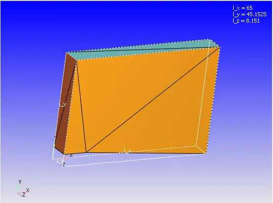
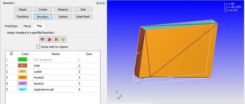
Each of the face is given a boundary name and allotted an ID.
The throttle is placed inside the elbow body
Since this is a steady state problem, the procedure to setup it is shown in the steps below.
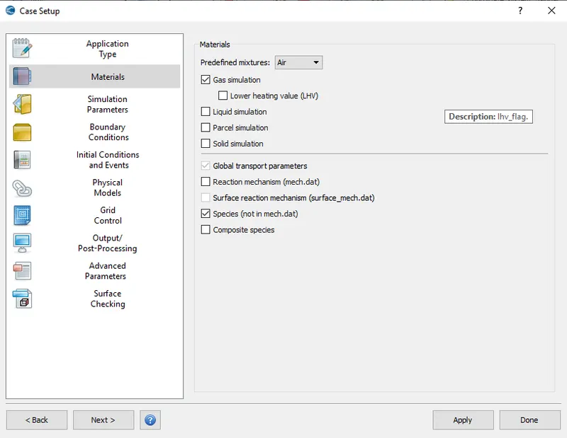
In the materials tab "Air" is selected and species tab is checked.
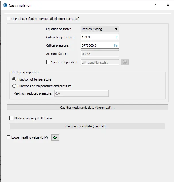
In the Gas simulation tab, default settings are set
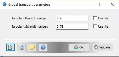
In the Global transport Parameters, defaults are kept to be same.
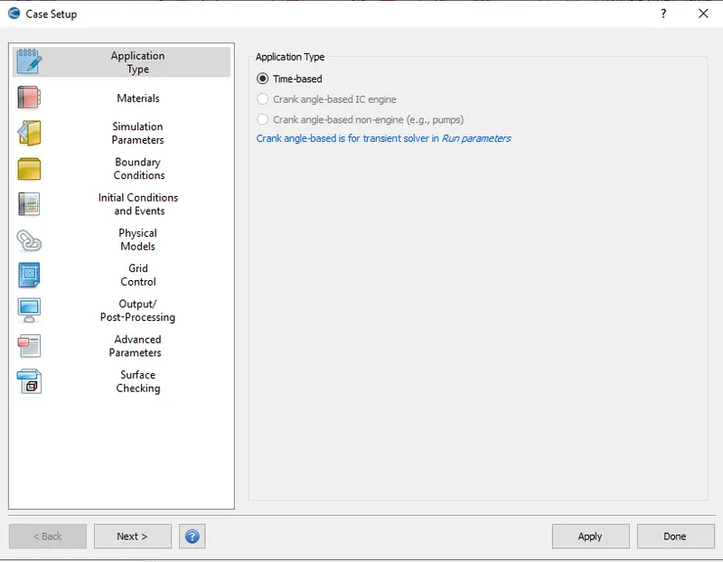
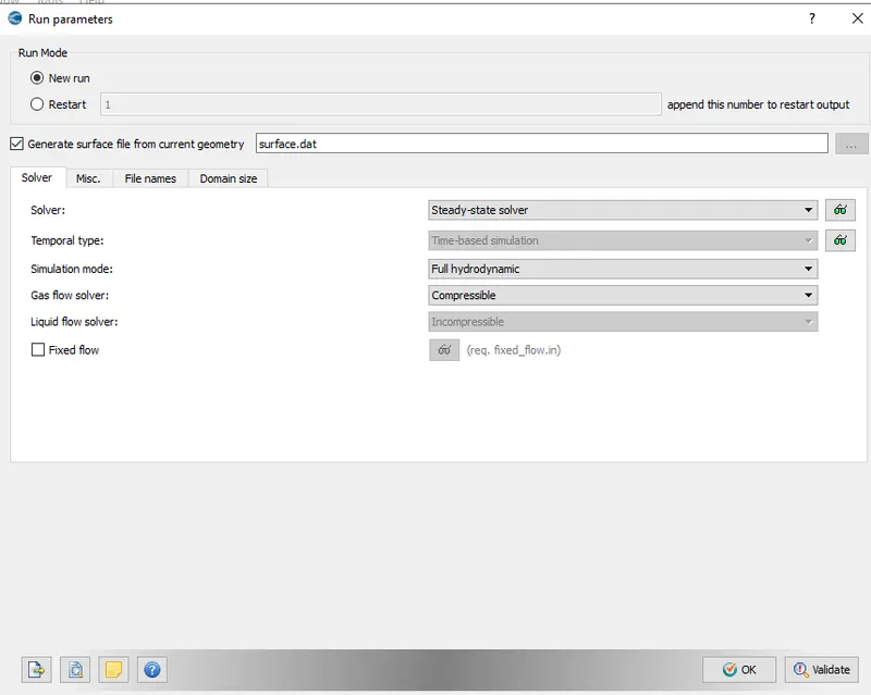
In the Run parameters tab, steady state solver is selected along with simulation mode to be in full hydrodynamic and solver used to be compressible.
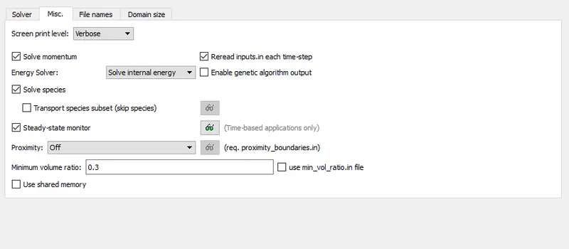
Also in the misc tab, steady state monitor is turned on for the convergence of results and shared memory tab is made off.
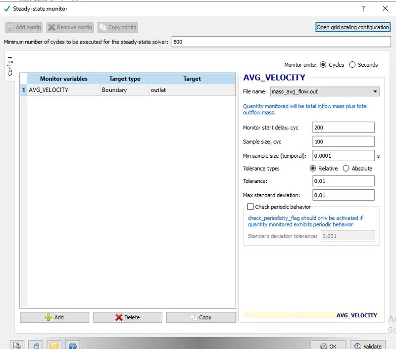
Average velocity monitor variables is selected.
The minimum number of cycles to be executed for steady state solver are set at 10000.
monitor start delay and sample size are set at 200 and 1000 respectively, as shown below.
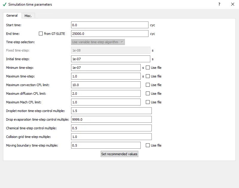
In the time parameters tab, end time is set to be at 15000 cycles and initial, minimum time steps to be 1e-09 and maximum time step is set at 1s.
PISO scheme is selected for solving the navier stokes equation and other values are set to be at the default.
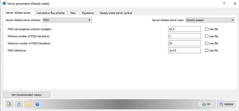
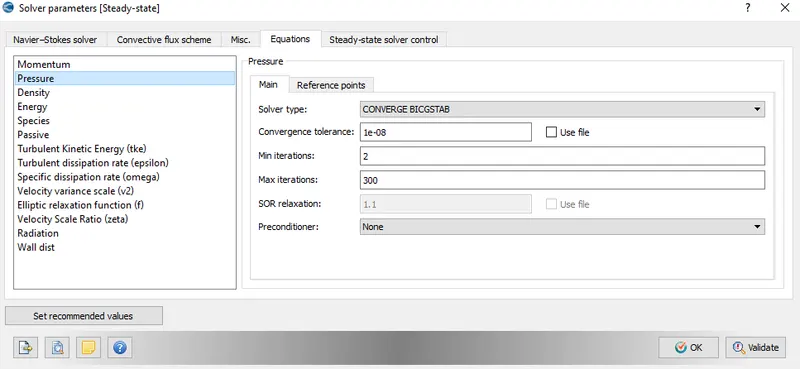
In these parameters, pressure term's precondition is set to be none.
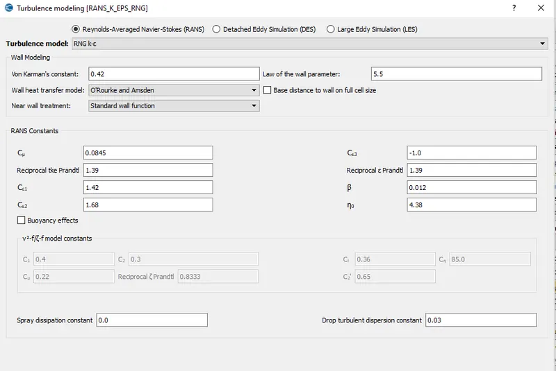
For the turbulence modelling RNGk-ε model is chosen with default values.
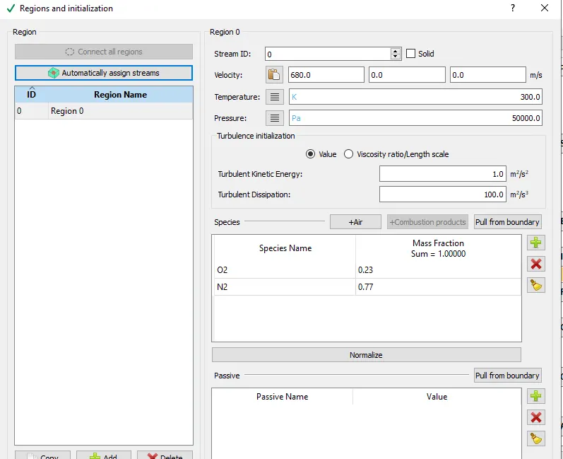
For initialization, a zone of different gases with unity summation of mass fractions and arbitrary values is set.
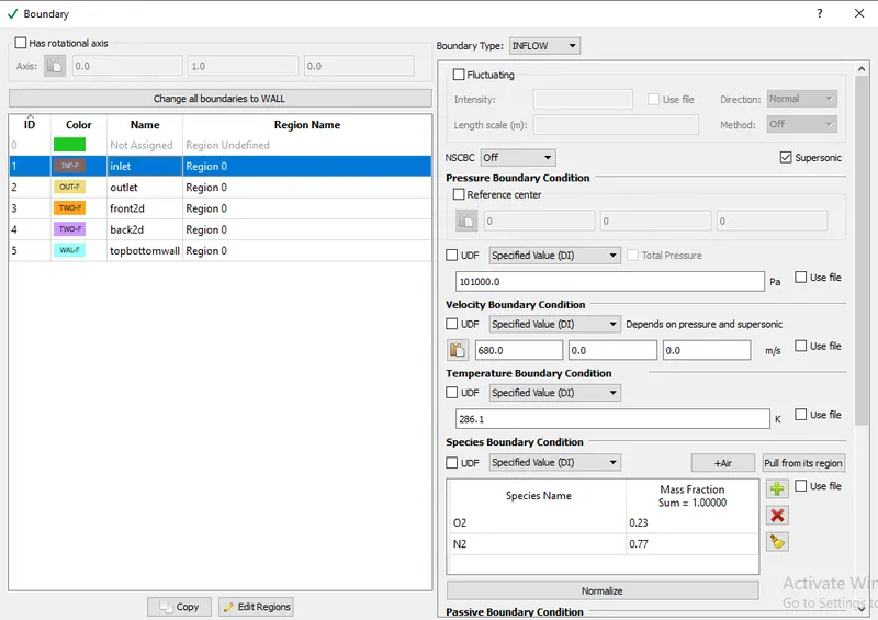
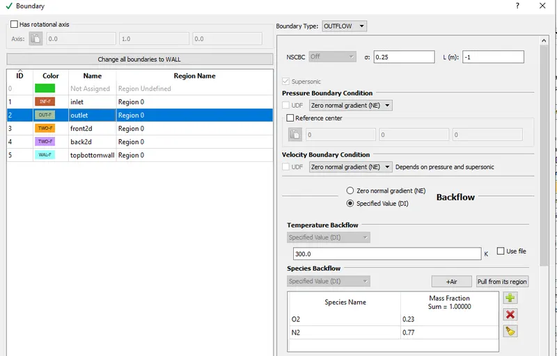
Futher the type of boundary and zone is set to all. Throttle is kept to be a non moving fixed wall. While the inlet and outlet pressures are kept at 150000 Pa and 100000 Pa respectively.
Grid sizing:
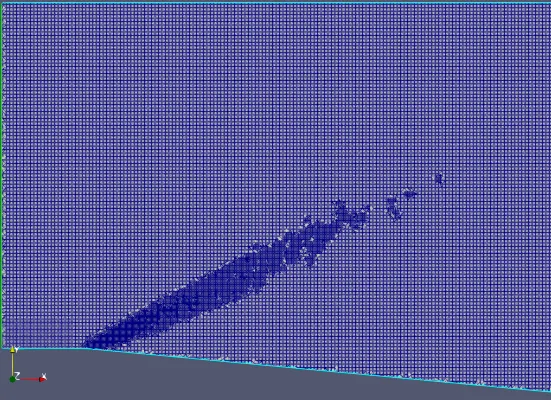
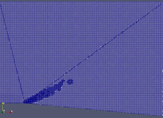
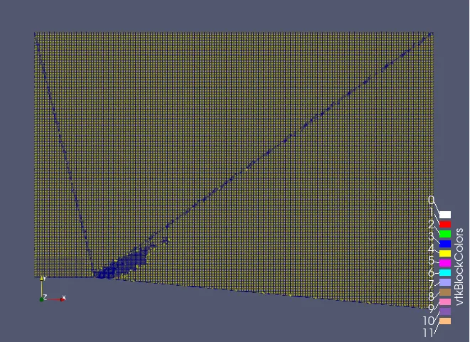
Grid of size 0.8 m is applied in all directions. Adaptive mesh refinement is applied with sub-grid criterion.
| Mesh.no. | dx-dy-dz | Sub-grid criterion |
| 1. | 0.8 | 0.05 |
| 2. | 0.8 | 0.07 |
| 3. | 0.8 | 0.1 |
Mesh 1-
Mesh 2-
Mesh 3-
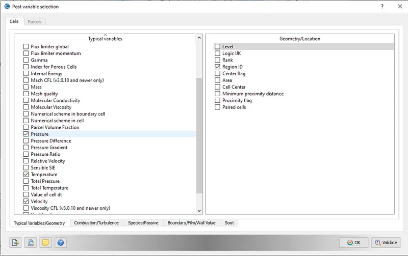
For getting the output values the required entities are selected.
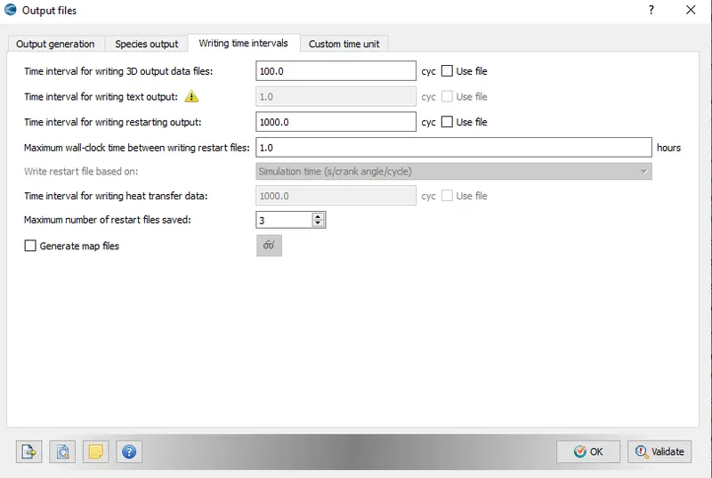
Number of cycles for 3d output data is set to be 100 cycles.
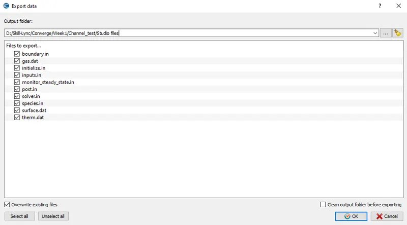
Finally the data files are exported which are solved by using the solver.
The input files are solved by using the cygwin.
Output:
Mesh 1
Mesh animation:
Final temperature contour:
Pressure contour:
Pressure animation:
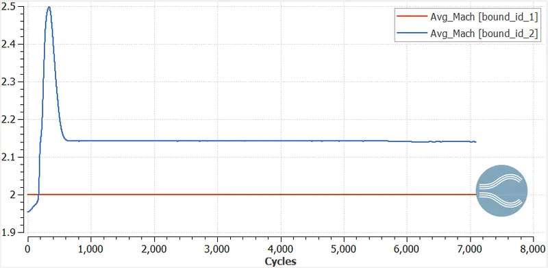
Plot for Mach number:
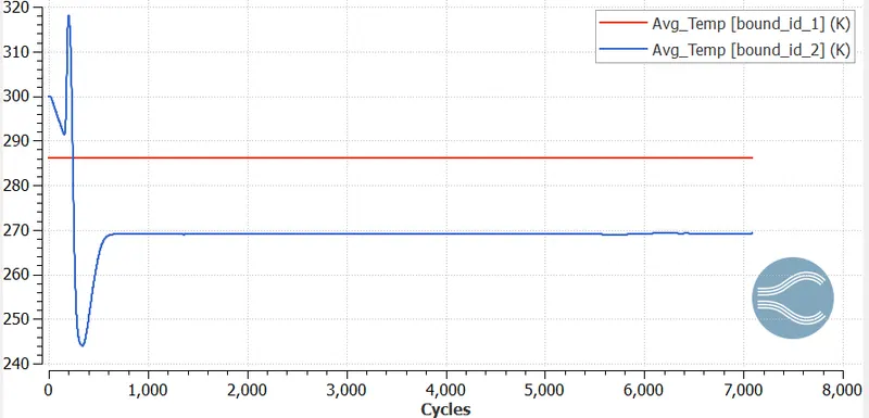
Plot for Average temperature:
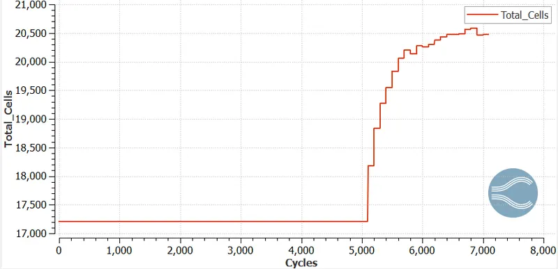
Plot for number of cells:
Mesh 2
Mesh animation:
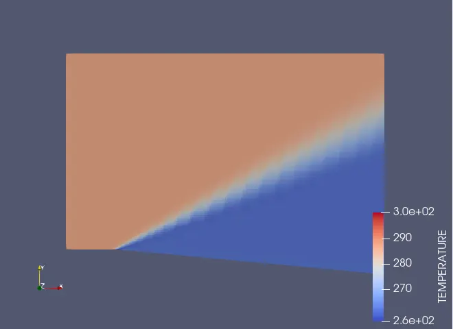
Final temperature contour:
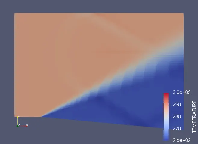
Temperature animation:
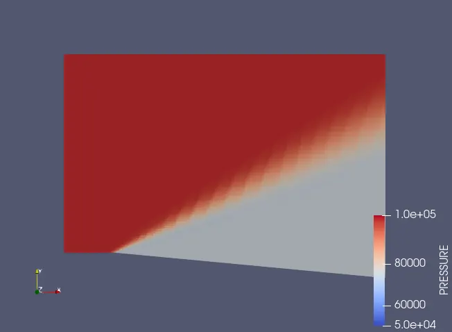
Pressure contour:
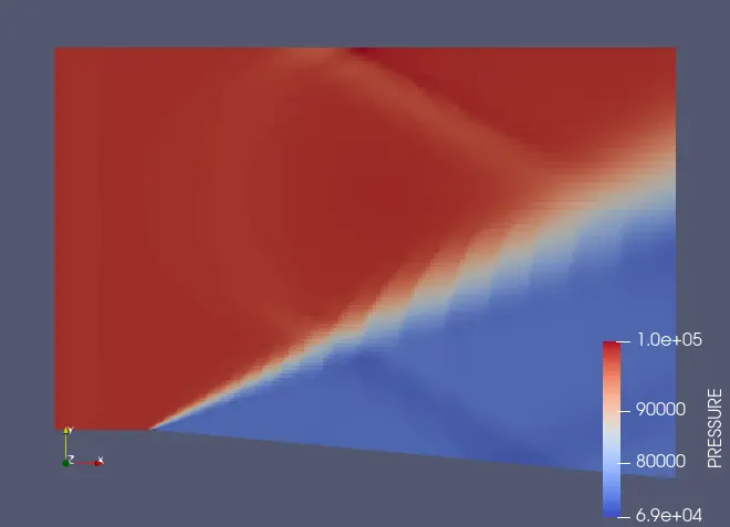
Pressure animation:
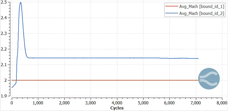
Plot for Mach number:
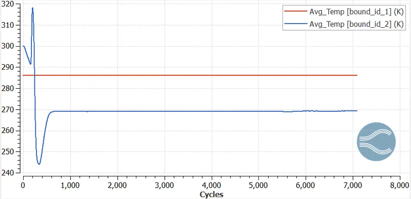
Plot for Average temperature:
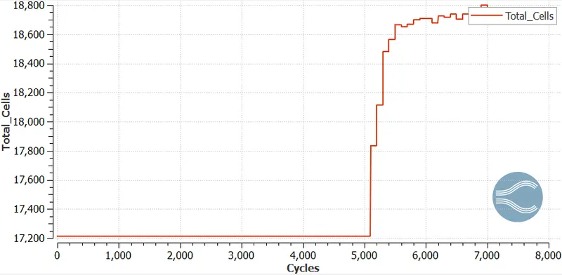
Plot for number of cells:
Mesh 3
Mesh animation:
Final temperature contour:
Temperature animation:
Pressure contour:
Pressure animation:
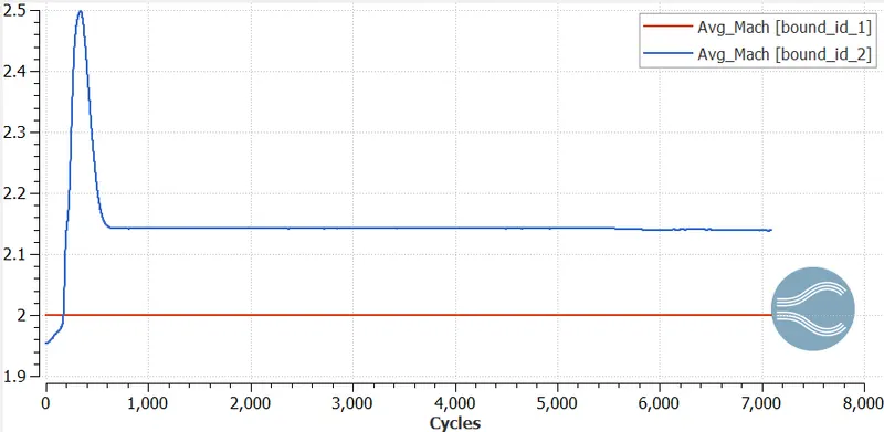
Plot for Mach number:
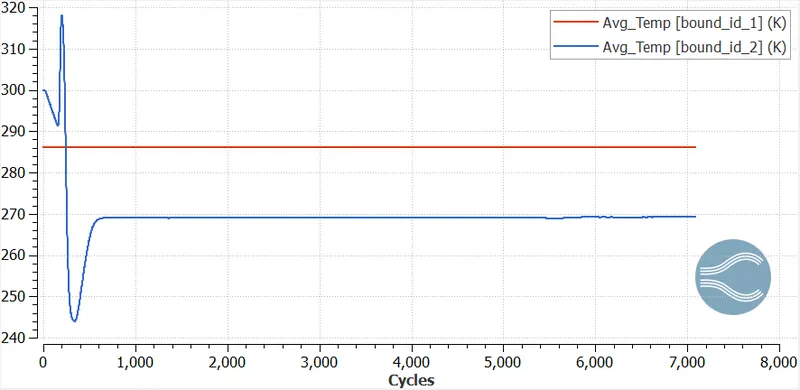
Plot for Average temperature:
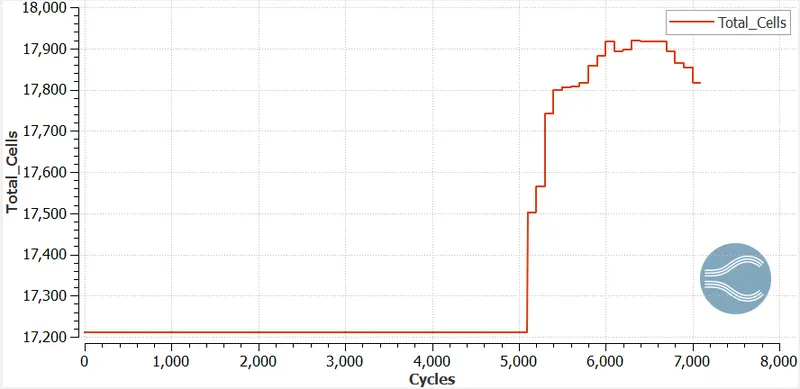
Plot for number of cells:
Conclusions:
- As the value of SGS in the adaptive meshing is decreased, the solution accuracy increases, hence the simulation time also increase.
- The SGS value of 0.05 gives the best result as it able to capture the minute details around the shock wave.
- Prandtl-Meyer Expansion fan works with the inlet mach number of 2 which is acheived through inner region and inlet boundary condition.
- There is large diiference in the number of cells at different SGS, as it increases with decrease in value of SGS.