Week 4.2: Project - Transient simulation of flow over a throttle body

Aim:

Setup and run transient state simulation for flow over a throttle body.

Post process the results and show pressure and velocity contours.

Show the mesh (i.e surface with edges)

Show the plots for pressure, velocity, mass flow rate and total cell count.

Also show the calculations on how you calculated an end time for the simulation.

Create an animation in which it throttle movement should be visible.

• Upload an animation on You tube and provide the You tube link for an animation in your report.

Introduction:

The throttle body is an important part of the air intake system that controls the air flowing into the engine. It’s located between air intake and engine manifold where fresh air is pulled into the engine for the combustion process. The amount of air allowed into the engine during this process controlled by the butterfly valve. The butterfly valve is a pivoting flat valve controlled by the gas pedal via cable or wire if controlled electronically. When pressing the peddle, the throttle body opens to allow more air flow into the manifold. The computer inside the vehicle works with sensors to ensure that the engine receives the perfect balance of fuel and air.

Filth, carbon, and dirt can build up in the housing creating problems with air flow. Known as coking, the normally smooth service for air to travel becomes full of gunk and creates an imbalance. This interrupts that perfect mixture of air and fuel which can cause the butterfly valve to get stuck. A stuck valve can cause surging or even stalling. This is why it’s important to have a good air filter for the vehicle. A fresh filter helps prevent dirt buildup on the surface of the butterfly valve. Poor idling or stalling when coming to a stop is another sign that may have an issue with the throttle body.

Modelling the problem in Converge Software

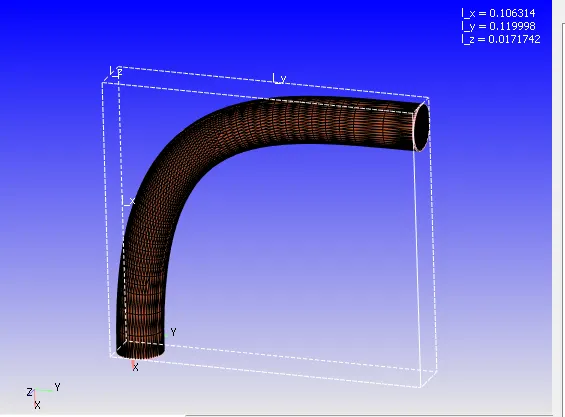
The 3D model is imported in the software.

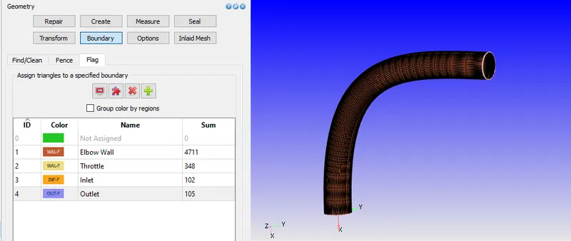
Each of the face is given a boundary name and allotted an ID.

The throttle is placed inside the elbow body

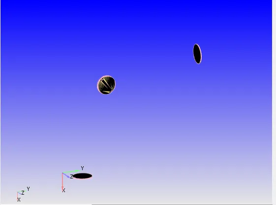
After this normal orientation is checked and then changed to the normal pointing inward to the body.

Since this is a Transient problem, the procedure to setup it is shown in the steps below.

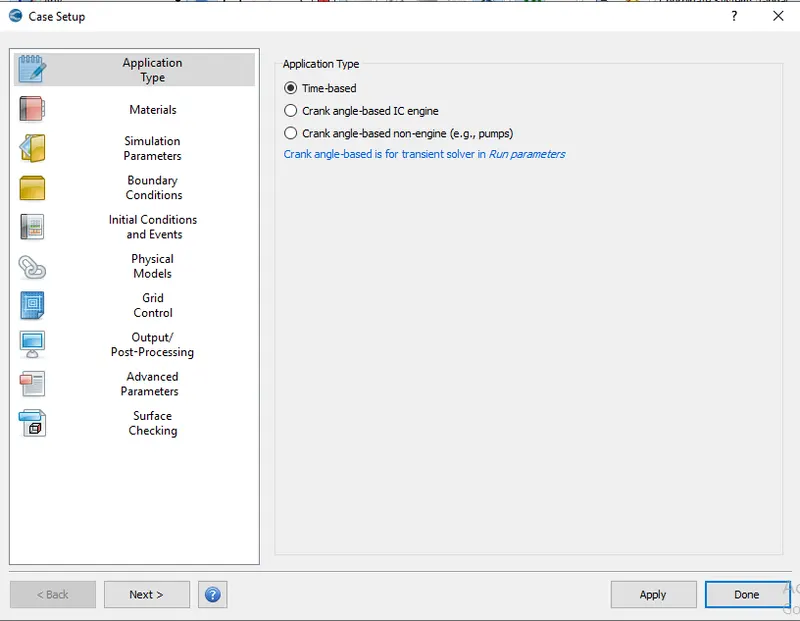
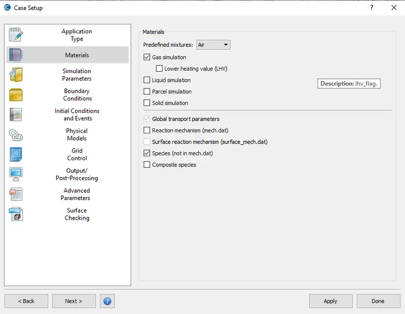
In the materials tab "Air" is selected and species tab is checked.

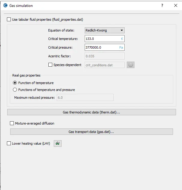
In the Gas simulation tab, default settings are set

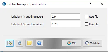
In the Global transport Parameters, defaults are kept to be same.

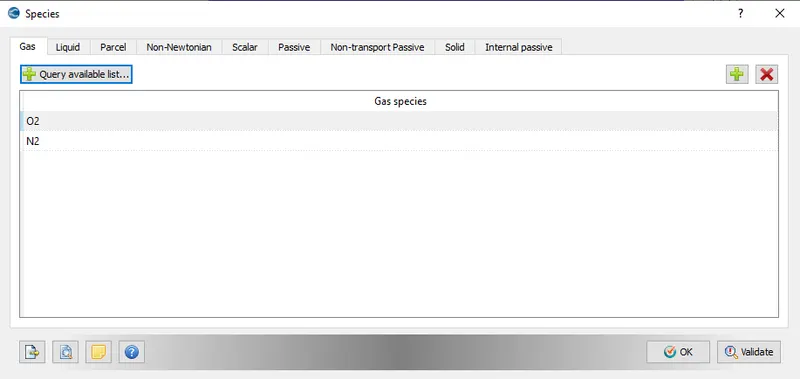
Oxygen and Nitrogen species are added in the species tab.

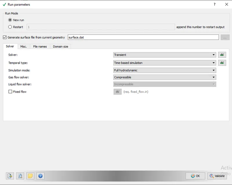
In the Run parameters tab, transient solver is selected along with simulation mode to be in full hydrodynamic and solver used to be compressible.

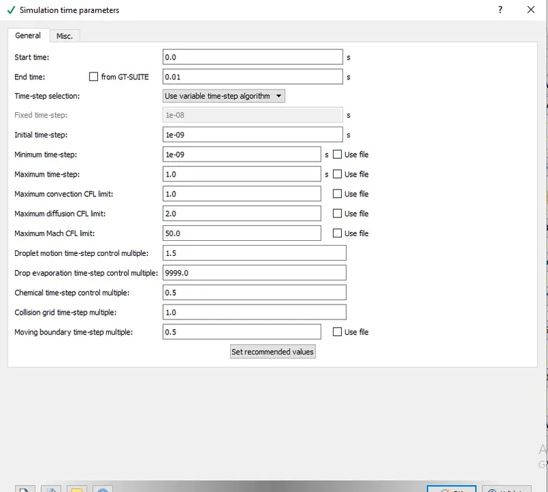
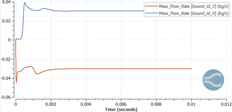
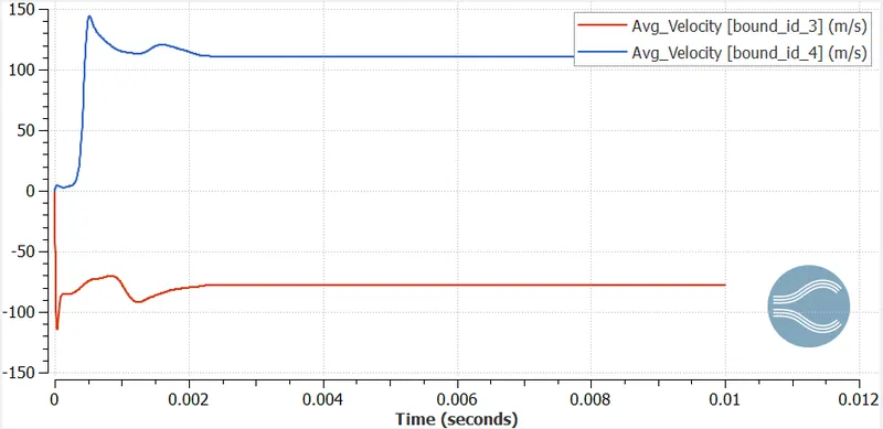
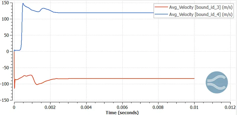
From the steady state analysis, it can be observed that the avg velocity after steady state is close to 100 m/s and the avergae length of the elbow is estimated to be 0.2m. So time taken for one flow pass is about 0.002 sec. for such 5 passes End time is taken as 0.01sec.

In the time parameters tab, minimum time steps to be 1e-09 and maximum time step is set at 1s.

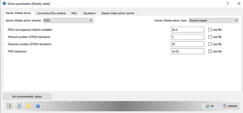
PISO scheme is selected for solving the navier stokes equation and other values are set to be at the default.

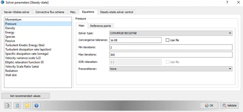
In these parameters, pressure term's precondition is set to be none.

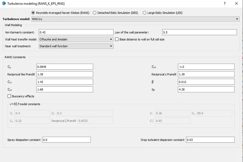
For the turbulence modelling RNG k-εmodel is chosen with default values.

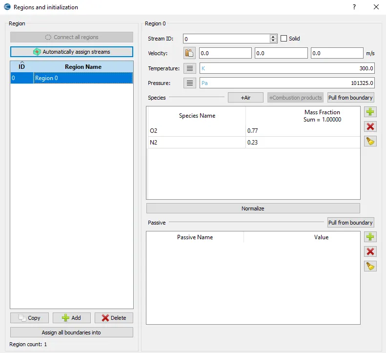
For initialization, a zone of different gases with unity summation of mass fractions and arbitrary values is set.

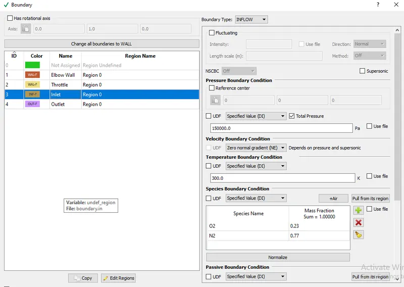
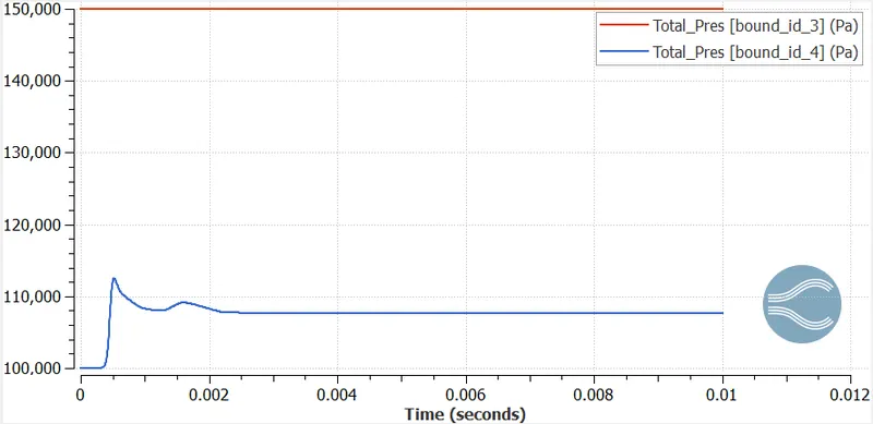
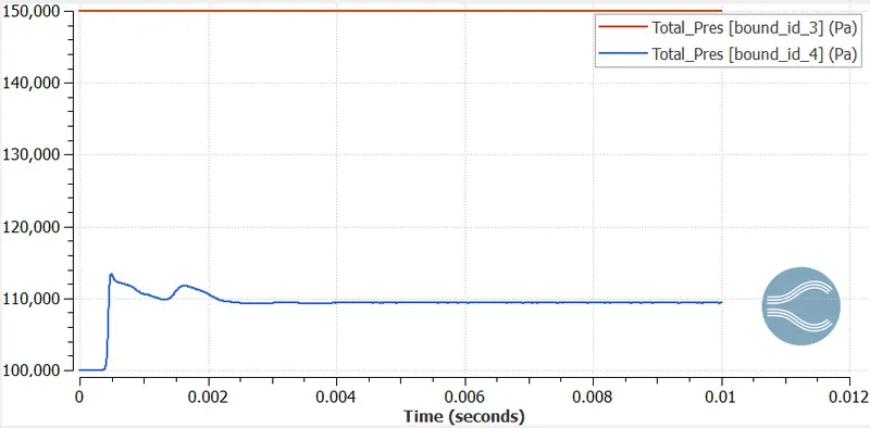
Futher the type of boundary and zone is set to all. Throttle is kept to be a moving fixed wall. While the inlet and outlet pressures are kept at 150000 Pa and 100000 Pa respectively.

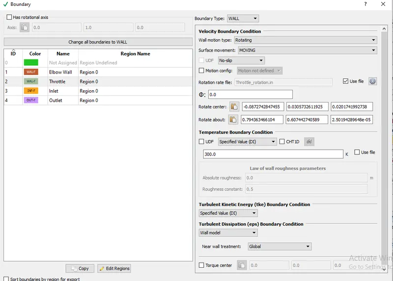
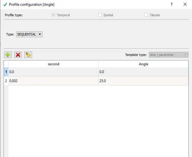
throttle roates about its axis whose parameters are given and it rotates by 25 degree after 0.002 sec.

Grid sizing:

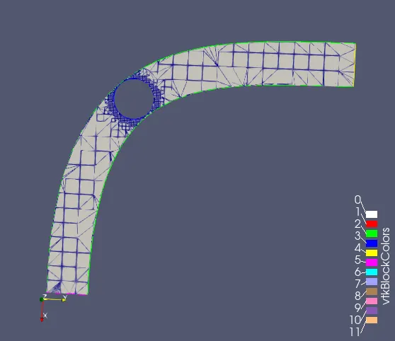
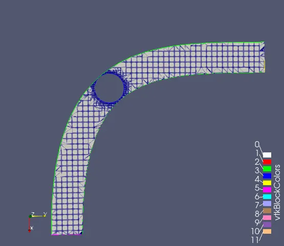
3 different size of grid are selected which are.

Mesh.no.	dx	dy	dz
1.	0.006	0.006	0.006
2.	0.003	0.003	0.003

Along with this grid size, fixed embracing is set at the Throttle walls with the scale factor of 3 and ebedded layers to be 2, to make the mesh more finer in this area.

Mesh 1-

Mesh 2-

For getting the output values the required entities are selected.

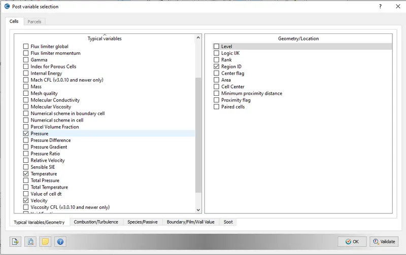
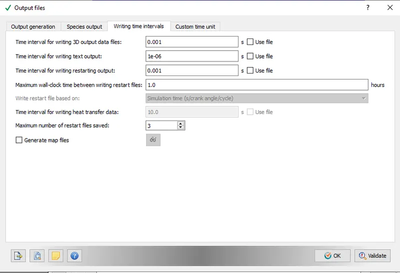
Ouput files are set as below.

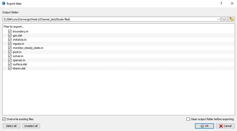
Finally the data files are exported which are solved by using the solver.

The input files are solved by using the cygwin.

Output:

Mesh 1

Mass Flow Rate plot at Inlet and Outlet-

Average velocity plot at Inlet and Outlet-

Total pressure plot at Inlet and Outlet-

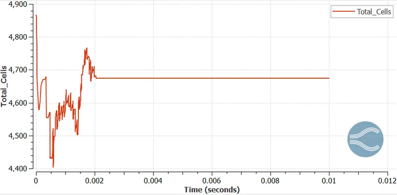
Total Number of cells plot-

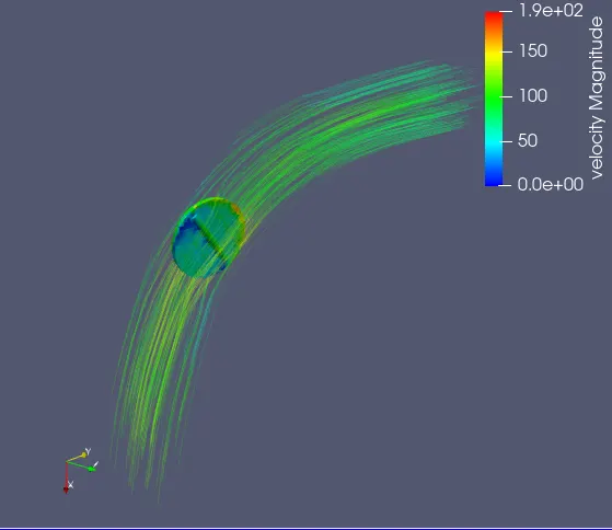
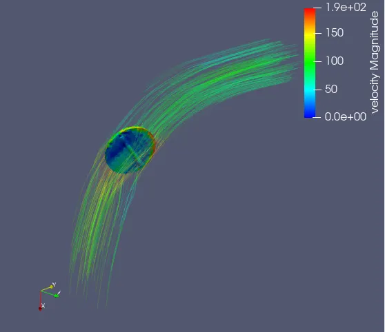
Streamlines-

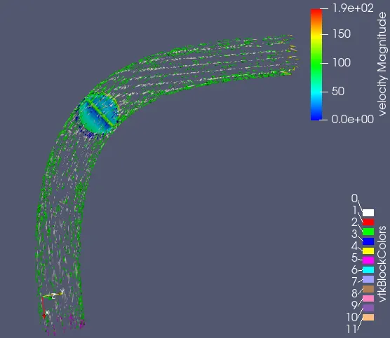
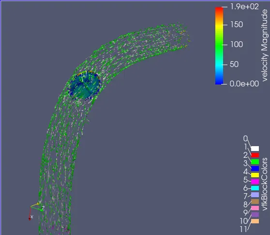
Velocity animation-

Pressure animation-

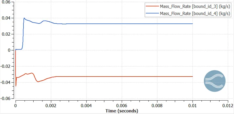
Mesh 2

Mass Flow Rate plot at Inlet and Outlet-

Average velocity plot at Inlet and Outlet-

Total pressure plot at Inlet and Outlet-

Total Number of cells plot-

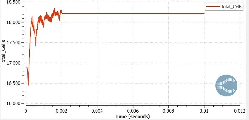
Number of cells change as the throttle is rotating with time.

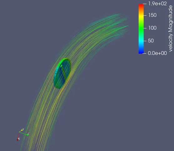
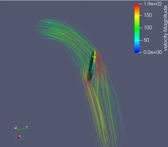
Streamlines-

Initially:

Finally:

Velocity animation-

Pressure animation-

Conclusions:

• As the mesh size is reduced the variation in the velocity is captured very accurately near the throttle body.
• The used turbulence model is accurate in predicting this problem.
• Due to the introduction of fixed embedding, flow behaviour is accurately achieved near the boundary.
• Stagnation point point is created in the localised area.
• The roatation of the throttle leads to the creation of turbulence in the area and is also observed in the streamline plots.
• Nomber of cells change as the throttle is moving and is depicted in the cell plot.