Week 3: Flow over a backward facing step

AIM

1. To set up a case of backward facing step in converge 3.0 software.

2. To use 3 different sizes of mesh for the problem.

3. Show the mesh (i.e surface with edges) for all the 3 base mesh sizes

4. Show pressure and velocity contours

5. Show the plots of velocity, pressure, mass flow rate and total cell count for all the 3 base mesh sizes

6. Also explain where and why separation is taking place in detail.

Backward Facing Step (BFS) is widely known for its application in the studies of turbulence in internal flows. The flow separation is caused due to the sudden changes in the geometry. This creates a zone of re-circulation and a point of flow reattachment. The physics of separated flows, due to their instabilities, are very complex. In an attempt to simplify these flow characteristics, researchers conducted experiments on various geometries, which include rib, fence, bluff body with a splitter plate, suddenly expanding pipes, forward and backward-facing steps, cavities, and bluff bodies with blunt leading edges. These geometries simplify the flow characteristics to a certain extent by fixing the separation or the reattachment point or both, which are otherwise unsteady. The backwards-facing step is considered by most the ideal canonical separated flow geometry because of its single fixed separation point and the wake dynamics unperturbed by the downstream disturbances. An illustration of the wake characteristics behind a backwards-facing step is shown in the Figure below

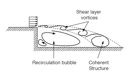
The flow behind the backward-facing step (BFS) is complex and involves various instability mechanisms. Based on the important flow features studied by previous researchers in a planar BFS geometry, the flow wake can be distinguished into three main regions namely, the shear layer region, separation bubble or recirculation zone and the reattachment zone. The general characteristics of a BFS flow begin with an upstream boundary layer separating at the step edge due to the adverse pressure gradient that develops into a thin shear layer (as shown in the figure below).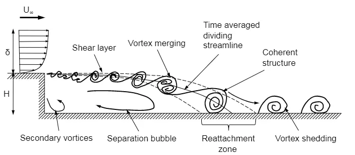

As the flow progresses downstream, the shear layer grows in size with the amalgamation of the turbulent structures contained within. This region where the shear layer develops and grows is referred to as the shear layer region. The turbulent structures in the shear layer entrain irrotational fluid from the non-turbulent region outside the shear layer. This flow entrainment causes the formation of a low-velocity recirculation in the region, which is located between the shear layer and the adjacent wall. The recirculation zone is mainly comprised of a primary vortex in the centre and a secondary vortex adjacent to the corner of the step.

Modelling the problem in Converge Software

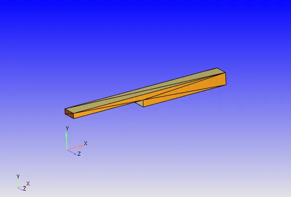
The 3D model is imported in the software.

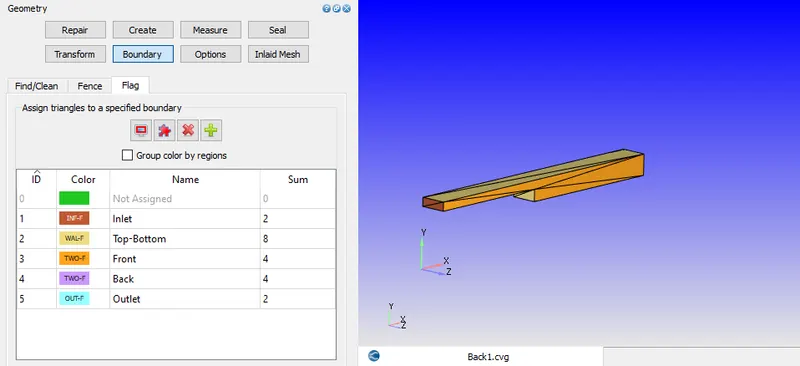
Each of the face is given a boundary name and allotted an ID.

After this normal orientation is checked and then changed to the normal pointing inward to the body.

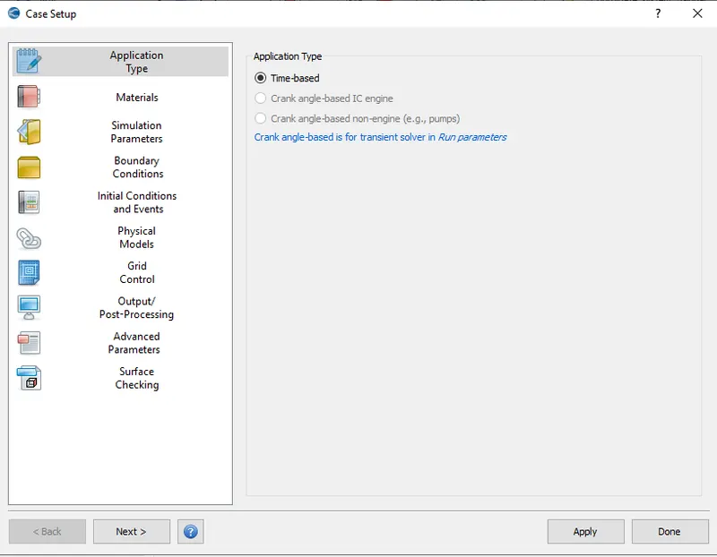
Since this is a steady state problem, the procedure to setup it is shown in the steps below.

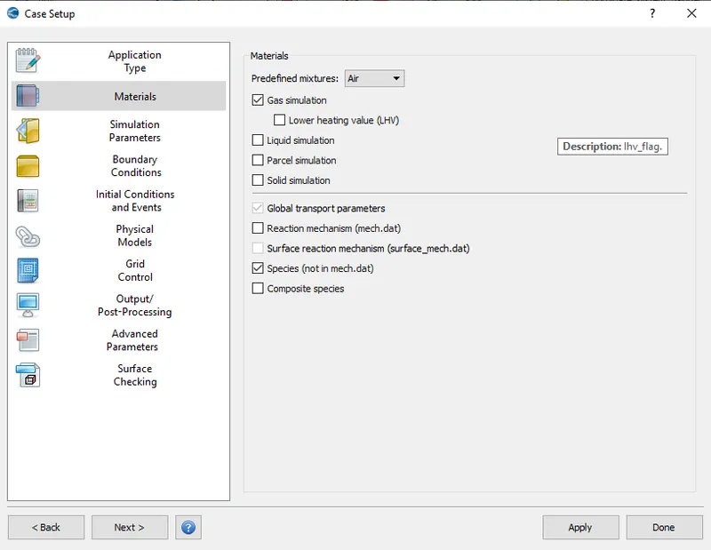
In the materials tab "Air" is selected and species tab is checked.

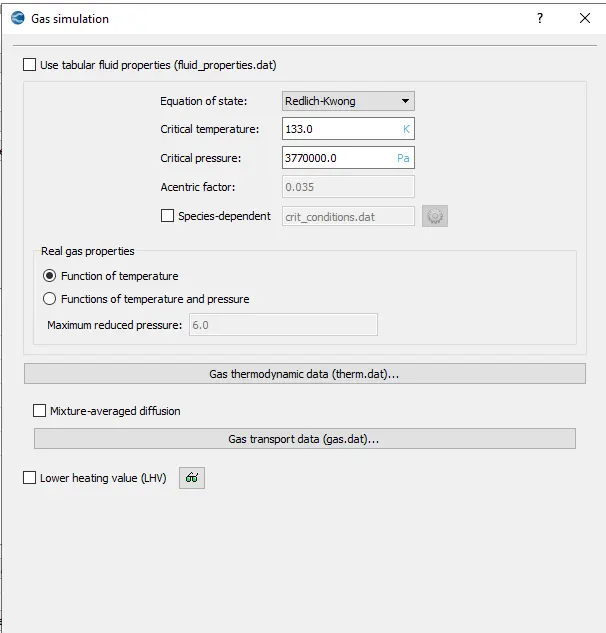
In the Gas simulation tab, default settings are set

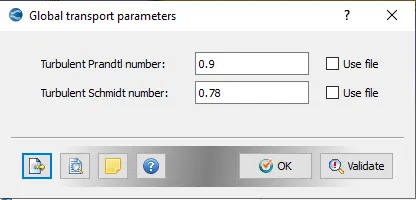
In the Global transport Parameters, defaults are kept to be same.

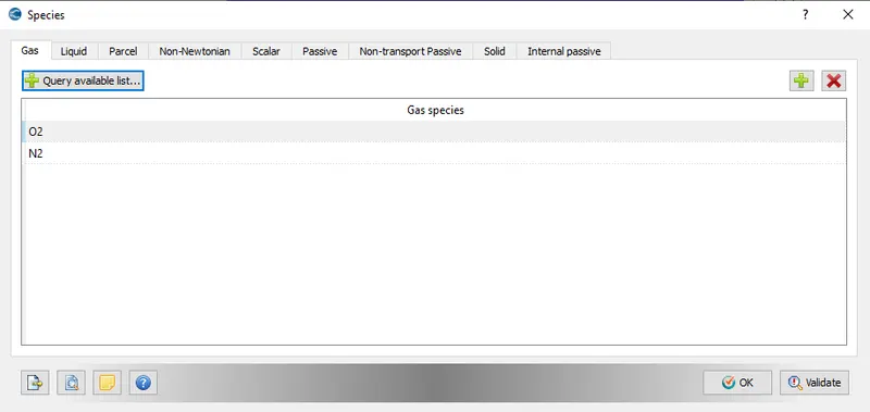
Oxygen and Nitrogen species are added in the species tab.

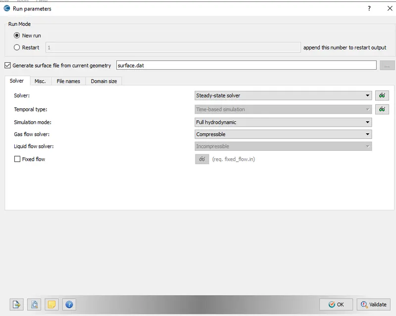
In the Run parameters tab, steady state solver is selected along with simulation mode to be in full hydrodynamic and solver used to be compressible.

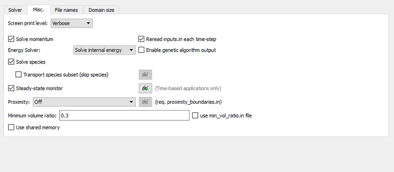
Also in the misc tab, steady state monitor is turned on for the convergence of results and shared memory tab is made off.

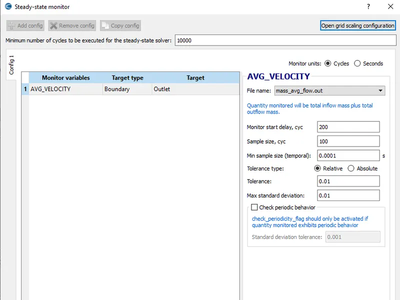
Average velocity monitor variables is selected.

The minimum number of cycles to be executed for steady state solver are set at 10000.

monitor start delay and sample size are set at 200 and 1000 respectively, as shown below.

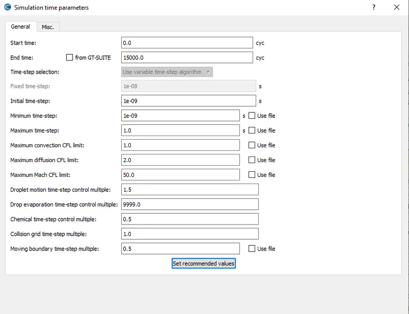
In the time parameters tab, end time is set to be at 15000 cycles and initial, minimum time steps to be 1e-09 and maximum time step is set at 1s.

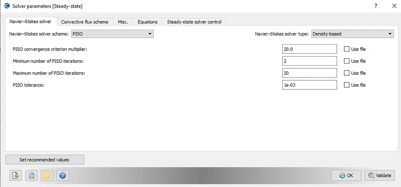
PISO scheme is selected for solving the navier stokes equation and other values are set to be at the default.

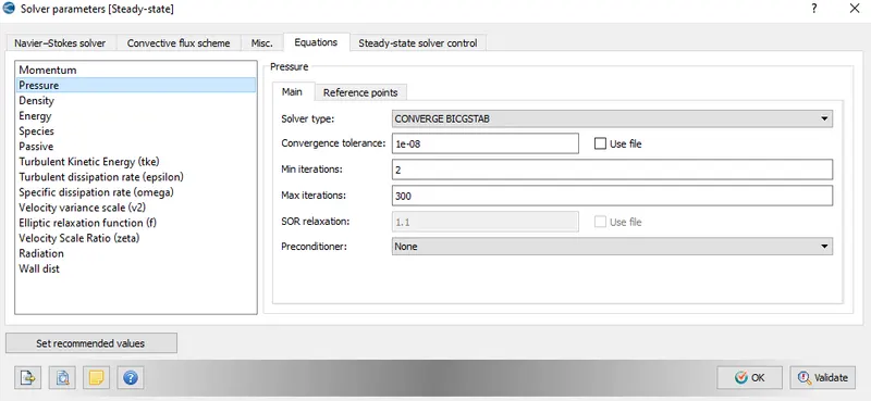
In these parameters, pressure term's precondition is set to be none.

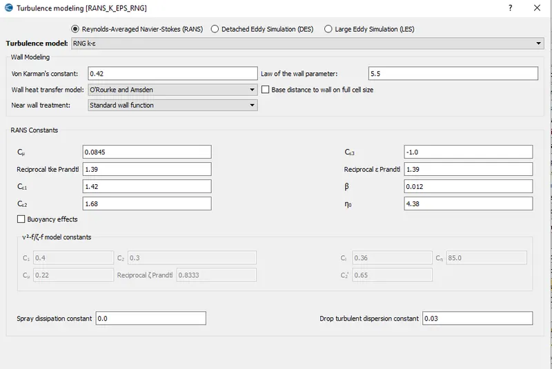
For the turbulence modelling `RNG k-epsilon`model is chosen with default values.

For initialization, a zone of different gases with unity summation of mass fractions and arbitrary values is set.

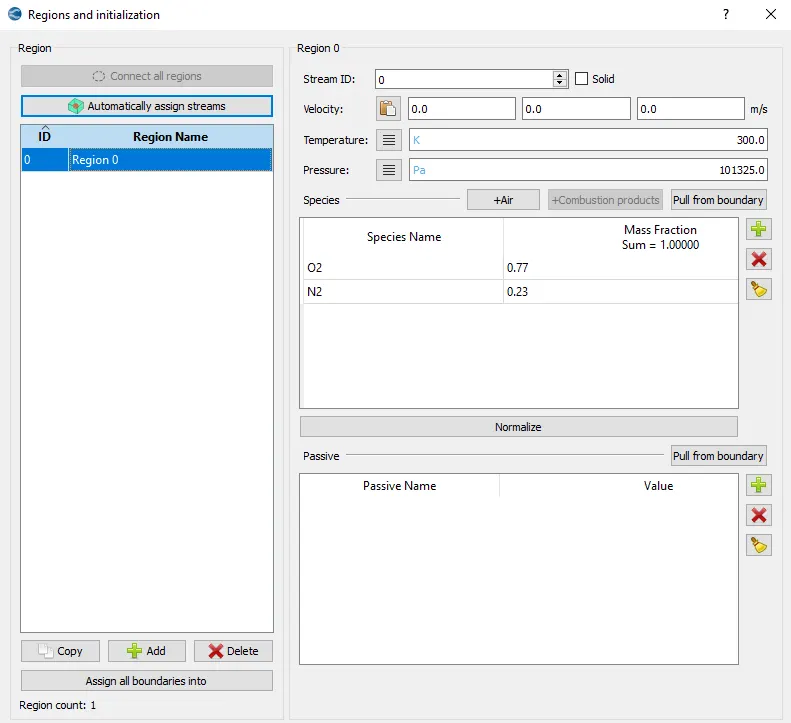
Futher the type of boundary and zone is set to all. Top and bottom faces are given a no slip condition, While others are defined the conditions as name states.

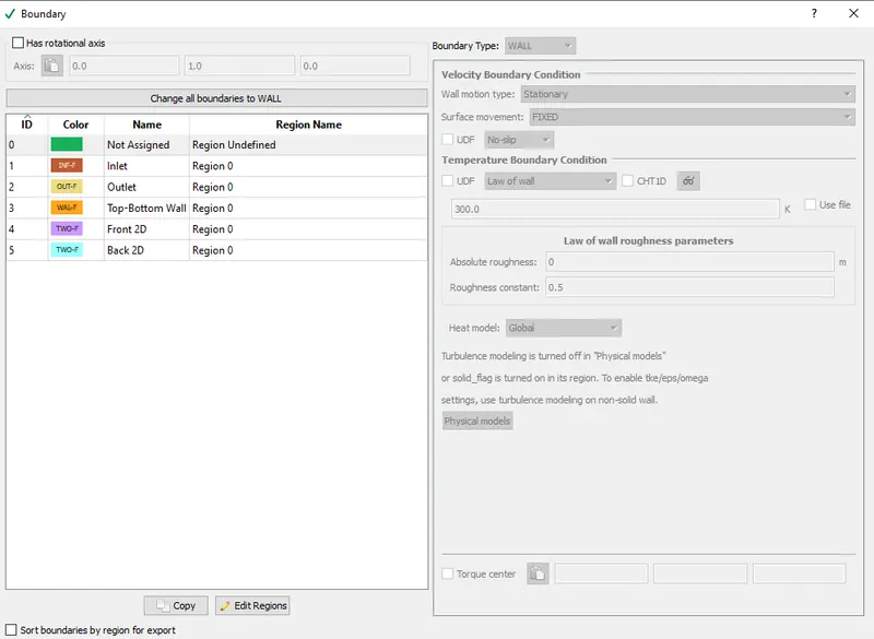
Inlet face is given a pressure of 110325 pa and outlet is set at 100325 pa.

Grid sizing:

3 different size of grid are selected which are.

Mesh.no.	dx	dy	dz
1.	0.002	0.002	0.002
2.	0.0015	0.0015	0.0015
3.	0.0012	0.0012	0.0012

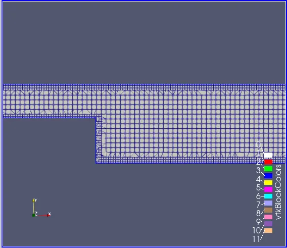
Along with this grid size, fixed embracing is set at the top and bottom walls with the scale factor of 1 to make the mesh more finer in these places

Mesh 1-

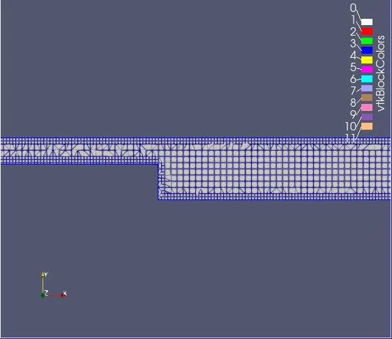
Mesh 2-

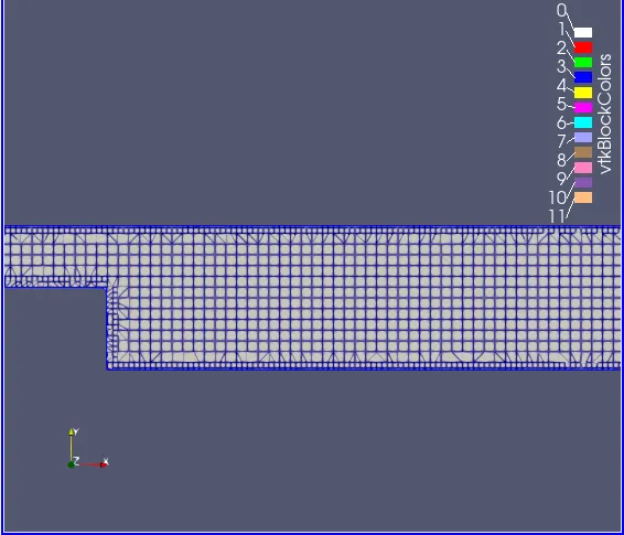
Mesh 3-

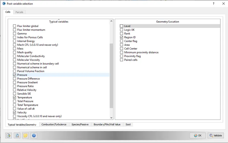
For getting the output values the required entities are selected.

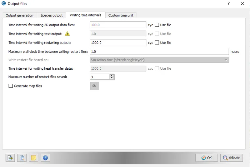
Number of cycles for 3d output data is set to be 100 cycles.

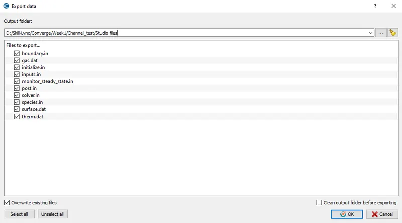
Finally the data files are exported which are solved by using the solver.

The input files are solved by using the cygwin.

Output:

Mesh 1

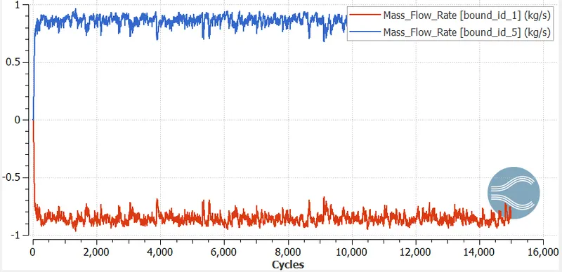
Mass Flow Rate plot at Inlet and Outlet-

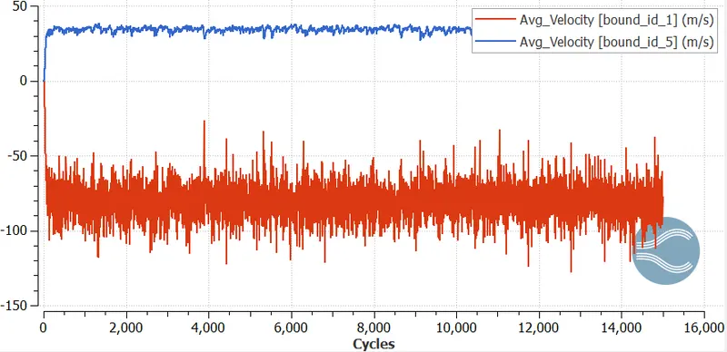
Average velocity plot at Inlet and Outlet-

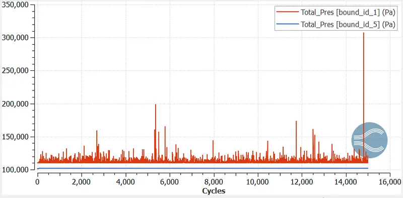
Total pressure plot at Inlet and Outlet-

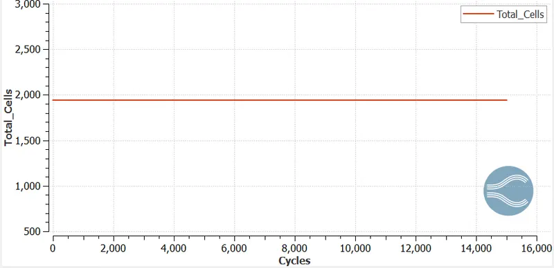
Total Number of cells plot-

Vector plot for coarse mesh-

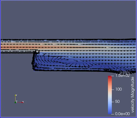
Velocity animation for coarse mesh-

Pressure animation for coarse mesh-

Mesh 2

Mass Flow Rate plot at Inlet and Outlet-

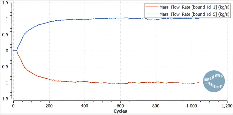
Average velocity plot at Inlet and Outlet-

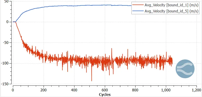
Total pressure plot at Inlet and Outlet-

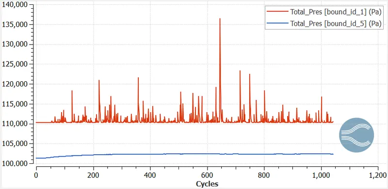
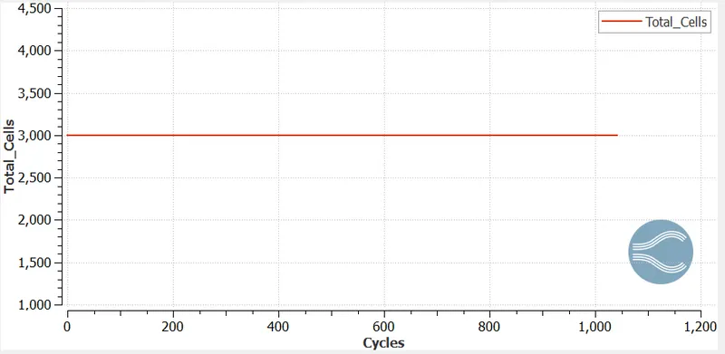
Totaal Number of cells plot-

Vector plot-

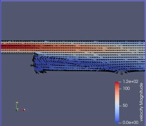
Velocity animation for medium mesh-

Pressure animation for medium mesh-

Mesh 3

Mass Flow Rate plot at Inlet and Outlet-

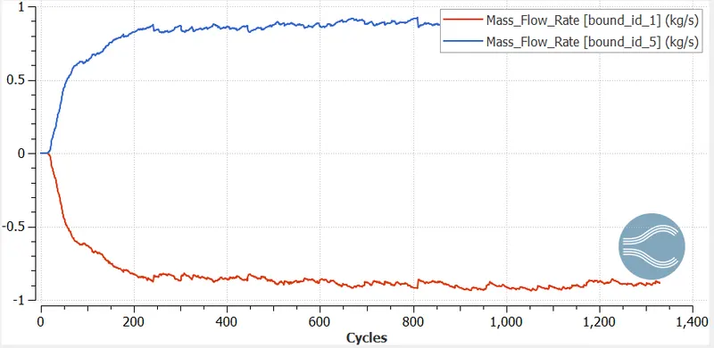
Average velocity plot at Inlet and Outlet-

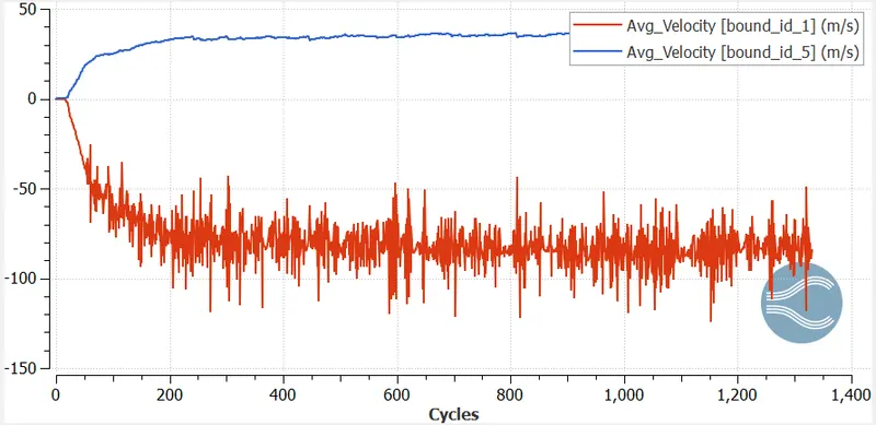
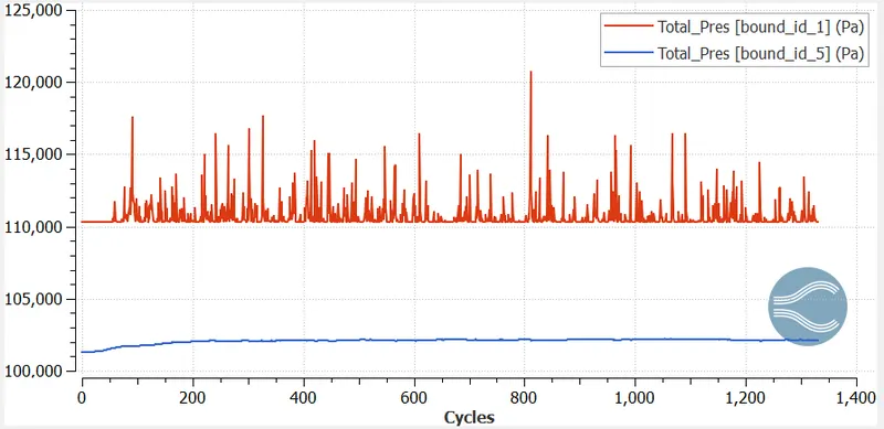
Total pressure plot at Inlet and Outlet-

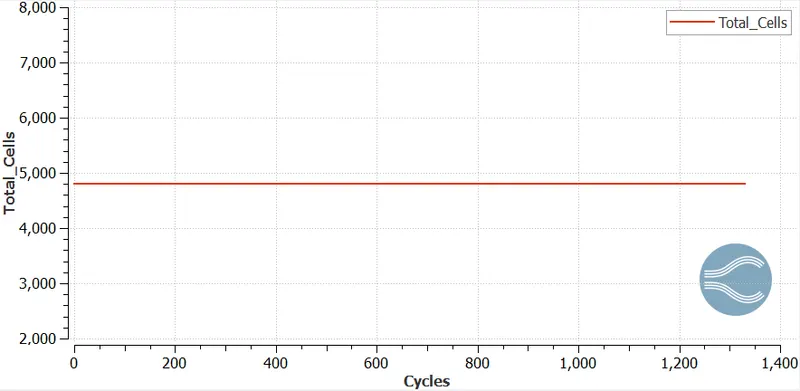
Total Number of cells plot-

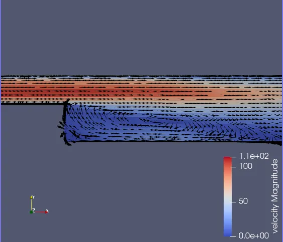
Vector plot-

Velocity animation for coarse mesh-

Pressure animation for coarse mesh-

Conclusions:

1. Thus, the steady-state solver is enough to visualize the flow in a backward step.
2. The used turbulence model i.e. `RNG k-epsilon`is good to model this complex problem.
3. As the mesh size is reduced the flow visualization can be seen to be improved.
4. There is the formation of eddies near the wall which ultimately leads to the phenomenon of flow separation.
5. The flow separation is occurring at the diverging location as due to phenomenon of no-slip. the fluid keeps in touch with the walls and is not able to fill up the entire vacant space when more area is present.

References:

(1) (PDF) On the flow characteristics behind a backward-facing step and the design of a new axisymmetric model for their study. Available from: https://www.researchgate.net/publication/266602855_On_the_flow_characteristics_behind_a_backward-facing_step_and_the_design_of_a_new_axisymmetric_model_for_their_study [accessed Aug 17 2022].

(2) Satheesh Kumar, A., Singh, A., & Thiagarajan, K. B. (2020, January). Simulation of backward facing step flow using OpenFOAM®. In AIP Conference Proceedings (Vol. 2204, No. 1, p. 030002). AIP Publishing LLC.