Week 7 - Auto ignition using Cantera

Auto ignition Temperature:

The autoignition temperature of a substance indicates the lowest temperature at which it may spontaneously ignite without the presence of an ignition source such as a flame or spark. At the auto-ignition temperature, the temperature alone provides sufficient energy to induce combustion. As the oxygen content of the ambient atmosphere increases, the auto-ignition temperature will decrease and increased pressure also decreases the temperature at which auto ignition can take place.

Ignition Delay:

Ignition delay time (IDT) is the time needed for a mixture of fuel and oxidizer to react at a certain temperature and pressure. This delay time is an important parameter for the engine designer and Ais typically determined experimentally. An experimental device capable of producing high-temperature and high-pressure conditions to perform such measurements is the shock tube.

PART I

• Plot the variation of Auto Ignition time of Methane with a constant temperature of 1250K and pressure varying from 1 to 5 atm.

The code for the problem is given as:

import sys
import numpy as np
import cantera as ct
import matplotlib.pyplot as plt

P_min = 1*101325
P_max = 5*101325
P=np.linspace(P_min,P_max,5)

for i in range(0,5):
	
	gas = ct.Solution('gri30.xml')
	T= 1250
	
	gas.TPX = T, P[i], {'CH4':1, 'O2': 2,'N2':7.52 }
	r= ct.IdealGasReactor(gas)
	sim = ct.ReactorNet([r])
	time = 0.0
	states = ct.SolutionArray(gas, extra =['time_in_ms', 't'])

	for n in range(10000):
		time +=1e-3
		sim.advance(time)
		states.append(r.thermo.state, time_in_ms = time*1e3, t = time)
	#print(states.T)
	plt.figure(1)
	plt.plot(states.t,states.T)
	
plt.legend(['1 atm','2 atm','3 atm','4 atm','5 atm'])
plt.show()

Output:

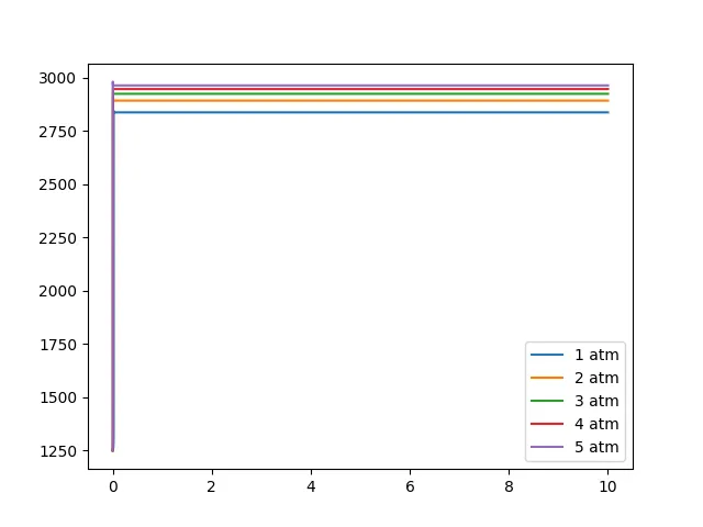
As the pressure is increased from 1 atm to 5 atm, auto-ignition temperature increases.

• Plot the variation of Auto Ignition time of Methane with a constant pressure of 5 atm and temperature varying from 950K to 1450K.

import sys
import numpy as np
import cantera as ct
import matplotlib.pyplot as plt

#T_min = 950
#T_max = 1450
T=[950,1050,1150,1250,1450]

for i in range(0,5):
	
	gas = ct.Solution('gri30.xml')
	
	P = 5*101325
	gas.TPX = T[i], P, {'CH4':1, 'O2': 2,'N2':7.52 }
	r= ct.IdealGasReactor(gas)
	sim = ct.ReactorNet([r])
	time = 0.0
	states = ct.SolutionArray(gas, extra =['time_in_ms', 't'])

	for n in range(10000):
		time +=1e-3
		sim.advance(time)
		states.append(r.thermo.state, time_in_ms = time*1e3, t = time)
	#print(states.T)
	plt.figure(1)
	plt.plot(states.t,states.T)
	
plt.legend(['950','1050','1150','1250', '1450'])
plt.show()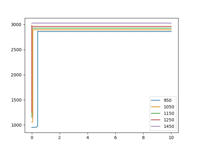

As the initial temperature is increased, auto-ignition temperature increases.

PART II

Further, observe and print the rate of change of molar concentrations of the given elements "H2O, O2, OH" with respect to the time, (simulation time = 10 secs)

Explain the behaviour of the graph for 2 cases,

• When Temperature is 1000K and pressure 5 bar

The code is given as:

import sys
import numpy as np
import cantera as ct
import matplotlib.pyplot as plt

gas = ct.Solution('gri30.xml')
T= 1000
P = 5*101325
gas.TPX = T, P, {'CH4':1, 'O2': 2,'N2':7.52 }
r= ct.IdealGasReactor(gas)
sim = ct.ReactorNet([r])
time = 0.0
states = ct.SolutionArray(gas, extra =['time_in_ms', 't'])

for n in range(10000):
	time +=1e-3
	sim.advance(time)
	states.append(r.thermo.state, time_in_ms = time*1e3, t = time)


#H2o
plt.subplot(1,3,1)
plt.plot(states.t,states.X[:,gas.species_index('H2O')])
plt.xlabel('Time in sec')
plt.legend(['H2O Molar Concentration'])
plt.title('H2O Variation')
plt.subplot(1,3,2)
plt.plot(states.t,states.X[:,gas.species_index('O2')])
plt.xlabel('Time in sec')
plt.legend(['O2 Molar Concentration'])
plt.title('O2 Variation')
plt.subplot(1,3,3)
plt.plot(states.t,states.X[:,gas.species_index('OH')])
plt.xlabel('Time in sec')
plt.legend(['OH Molar Concentration'])
plt.title('OH Variation')
plt.show()

Output:

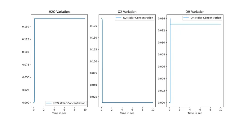
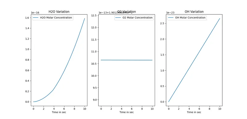
• When Temperature is 500K and pressure 5 bar

Code:

import sys
import numpy as np
import cantera as ct
import matplotlib.pyplot as plt

gas = ct.Solution('gri30.xml')
T= 500
P = 5*101325
gas.TPX = T, P, {'CH4':1, 'O2': 2,'N2':7.52 }
r= ct.IdealGasReactor(gas)
sim = ct.ReactorNet([r])
time = 0.0
states = ct.SolutionArray(gas, extra =['time_in_ms', 't'])

for n in range(10000):
	time +=1e-3
	sim.advance(time)
	states.append(r.thermo.state, time_in_ms = time*1e3, t = time)


#H2o
plt.subplot(1,3,1)
plt.plot(states.t,states.X[:,gas.species_index('H2O')])
plt.xlabel('Time in sec')
plt.legend(['H2O Molar Concentration'])
plt.title('H2O Variation')
plt.subplot(1,3,2)
plt.plot(states.t,states.X[:,gas.species_index('O2')])
plt.xlabel('Time in sec')
plt.legend(['O2 Molar Concentration'])
plt.title('O2 Variation')
plt.subplot(1,3,3)
plt.plot(states.t,states.X[:,gas.species_index('OH')])
plt.xlabel('Time in sec')
plt.legend(['OH Molar Concentration'])
plt.title('OH Variation')
plt.show()

Output: