Week 5 - Mid term project - Solving the steady and unsteady 2D heat conduction problem
1. Steady State Analysis:
Solving the 2D heat conduction equation by using the point iterative techniques that were taught in the class. The Boundary conditions for the problem are as follows;
Top Boundary = 600 K
Bottom Boundary = 900 K
Left Boundary = 400 K
Right Boundary = 800 K
The steady state heat equation can be represented by-
`delT^2//delx^2 + delT^2//dely^2 = 0`
Assume nx = ny
On solving the the above equation by using the Taylor series 2nd order results we get the equation for T as
`Tp = (K1 * (Tl + Tr)) + (k2* (Tt + Tb))`
where
`k1 = Delta y^2 // (2*(Deltax^2 + Deltay^2))`
`k2 = Delta x^2 // (2*(Deltax^2 + Deltay^2))`
Tl & Tr are the points on the left and right of our point of calculation
Tt & Tb are the points on the top and bottom of our point of calculation
The implicit schemes will be employed for solving the problems which are:
1. jacobi
2. Gauss Siedel
3. Succesive over Relaxation
The matlab code to calculate this is
clear all
close all
clc

nx = 10;
ny = 10;
L  = 1;
x = linspace(0,L,nx);
y = linspace(0,L,ny);

dx = x(2)-x(1);
dy = y(2) - y(1);

K1 = (dy^2/ (2*(dx^2 + dy^2)));
K2 = (dx^2/ (2*(dx^2 + dy^2)));
T = 100*ones(nx,ny);

T(2:nx-1,1) = 400;
T(2:nx-1,ny) = 800;
T(1, 2:ny-1) = 600;
T(nx, 2:ny-1) = 900;

T(1,1) = 500;
T(1,ny) = 700;
T(nx,1) = 650;
T(nx,ny) = 850;

T_old = T;
tol = 1e-4;
error = 9e9;


iter =3;

%Jacobi
if iter == 1;
    itt = 1;
    while (error>tol)
           for i = 2:nx-1
            for j = 2:ny-1
                T(i,j) = ((T_old(i-1,j) + T_old(i+1,j)) * K1)  + ((T_old(i,j-1) + T_old(i,j+1)) * K2);
            end
        end
        error = max(max(abs(T_old - T)));
        T_old = T;
        itt = itt+1;
    end

    figure(1)
    contourf(x,y,T, 'showText', 'on')
    colormap(jet)
    set(gca, 'Ydir', 'reverse')
    colorbar
    title_text = sprintf('Jacobi : Number of iterations : %d',itt);
    title(title_text)
end


% GS

if iter == 2;
    itt = 1;
    while (error>tol)
              for i = 2:nx-1
            for j = 2:ny-1
                T(i,j) = ((T(i-1,j) + T(i+1,j)) * K1)  + ((T(i,j-1) + T(i,j+1)) * K2);
            end
        end
        error = max(max(abs(T_old - T)));
        T_old = T;
        itt = itt+1;
    end

    figure(2)
    contourf(x,y,T, 'showText', 'on')
    set(gca, 'Ydir', 'reverse')
    colormap(jet)
    colorbar
    title_text = sprintf('Jacobi : Number of iterations : %d',itt);
    title(title_text)
end

%Successive over relaxation
w = 1.1;
if iter == 3;
    itt = 1;
    while (error>tol)
                for i = 2:nx-1
            for j = 2:ny-1
                T(i,j) = ((1-w)*T_old(i,j)) +(w * (((T(i-1,j) + T(i+1,j)) * K1)  + ((T(i,j-1) + T(i,j+1)) * K2))) ;
            end
        end
        error = max(max(abs(T_old - T)));
        T_old = T;
        itt = itt+1
    end

    figure(3)
    contourf(x,y,T, 'showText', 'on')
    set(gca, 'Ydir', 'reverse')
    colormap(jet)
    colorbar
    title('SOR')
    title_text = sprintf('Jacobi : Number of iterations : %d',itt);
    title(title_text)
end
The plots in result we are getting are -
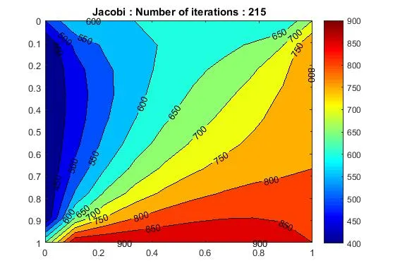
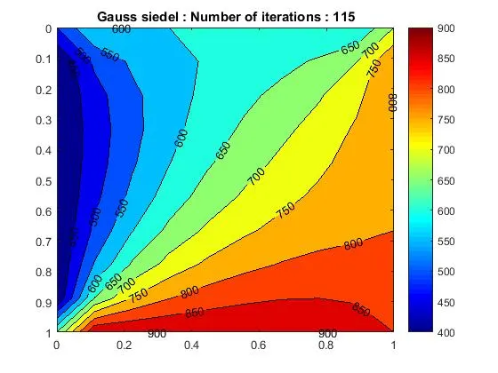
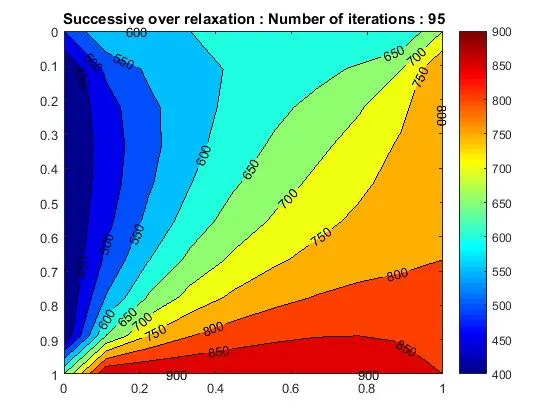
From the Above plots it is clearly observed that the Successive over relaxation method coverges to steady steady at very lesser number of iterations. Also it takes fewer time steps to solve the problem.
So we can observe that the no. of iterations are in order of
Successive Over Relaxation>Gauss Siedel >Jacobi
2. Solving 2D transient heat conduction equation(unsteady state):
The transient heat equation is given by-
`dT//dt = alpha * (d^2T//dx^2 + d^2T//dy^2)`
on seperating the above equation and then arranging as per time steps we get,
`Tp^(n+1) = Tp^n + K1*(Tl - 2*Tp +Tr)^n + K2*(Tt - 2*Tp + Tb)^n`
There are two ways to solve the problem:
a.) Explicit method
b.)Implicit method
a.)Exlplicit method-
The implicit metod is solved by using surrounding conditions and our point at the new time step .
The matlab code to solve the explicit method is
clear all
close all
clc

%Defining our mesh size and iput values
nx = 10;
ny = 10;
L  = 1;
x = linspace(0,L,nx);
y = linspace(0,L,ny);

dx = x(2)-x(1);
dy = y(2) - y(1);


%creating temperature inputs
T = 100*ones(nx,ny);

T(2:nx-1,1) = 400;
T(2:nx-1,ny) = 800;
T(1, 2:ny-1) = 600;
T(nx, 2:ny-1) = 900;

T(1,1) = 500;
T(1,ny) = 700;
T(nx,1) = 650;
T(nx,ny) = 850;

T_old = T;
tol = 1e-3;
error = 9e9;
dt = 1e-3;
alpha = 1;
%CFL number
%K1 = alpha*dt / dx^2;
%K2 = alpha*dt/ dy^2;
%K1 = K2 = K
K = alpha*dt/dx^2;
%for t= 1:10;
iter = 0;

while(error>tol)
    for i = 2:nx-1;
        for j = 2:ny-1;
            T(i,j) = (1-4*K)*T_old(i,j) + K*(T_old(i-1,j) + T_old(i+1,j) + T_old(i,j-1) + T_old(i,j+1));
        end
    end
    error = max(max(abs(T_old - T)));
    T_old  = T;
    iter = iter +1;

end
% Plotting graph
figure(2)
contourf(x,y,T,'showText','on')
set(gca,'Ydir','reverse')
colormap(jet)
colorbar
title_text = sprintf('Explicit method for Transient state, Number of iterations : %d',iter);
title(title_text)
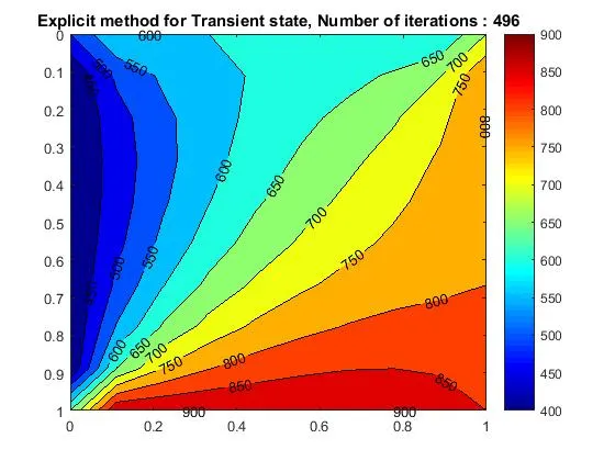
In the output we get the plot as,
b.)Implicit Method-
The implicit metod is solved by using surrounding conditions at the new time step and our point condition at older time step.
There are three methods to solve this-
1. Jacobi
2.Gauss Siedel
3. Successive over relaxation
clear all
close all
clc

%Defining our mesh size and iput values
nx = 20;
ny = 20;
L  = 1;
x = linspace(0,L,nx);
y = linspace(0,L,ny);

dx = x(2)-x(1);
dy = y(2) - y(1);


%creating temperature inputs
T = 100*ones(nx,ny);

T(2:nx-1,1) = 400;
T(2:nx-1,ny) = 800;
T(1, 2:ny-1) = 600;
T(nx, 2:ny-1) = 900;

T(1,1) = 500;
T(1,ny) = 700;
T(nx,1) = 650;
T(nx,ny) = 850;

T_old = T;
T_prev = T;
tol = 1e-4;
error = 9e9;
dt = 10;
alpha = 1.4;

%CFL number
K1 = alpha*dt / dx^2;
K2 = alpha*dt/ dy^2;
term1 = 1/(1+2*K1 + 2*K2);
term2 = K1 * term1;
term3 = K2 * term1;

s_iter = 0;
t_iter = 0;
conv = 9e9;

itt = 3;
%Jacobi
if itt == 1
    while(conv>tol)
        while (error>tol)
            for i = 2:nx-1
                for j = 2:ny-1
                    H = (T_old(i-1,j) + T_old(i+1,j));
                    V = (T_old(i,j-1) + T_old(i,j+1));
                    T(i,j) = term1*T_prev(i,j)+(H*term2) + (V*term3);
                end
            end
            error = max(max(abs(T_old - T)));
            T_old = T;
            s_iter = s_iter+1;
        end
        conv= max(max(abs(T_prev - T)));
        T_prev = T;
        t_iter = t_iter+1;
    end

    % Plotting graph
    figure(1)
    contourf(x,y,T, 'showText', 'on')
    set(gca, 'Ydir', 'reverse')
    colormap(jet)
    colorbar
    title_text = sprintf('Jacobi : Number of iterations in space and time: %d and %d',s_iter,t_iter);
    title(title_text)
end

%GS
if itt==2
    while(conv>tol)
        while (error>tol)
            for i = 2:nx-1
                for j = 2:ny-1
                    H = (T(i-1,j) + T_old(i+1,j));
                    V = (T(i,j-1) + T_old(i,j+1));
                    T(i,j) = term1*T_prev(i,j)+(H*term2) + (V*term3);
                end
            end
            error = max(max(abs(T_old - T)));
            T_old = T;
            s_iter = s_iter+1;
        end
        conv= max(max(abs(T_prev - T)));
        T_prev = T;
        t_iter = t_iter+1;
    end

    % Plotting graph
    figure(2)
    contourf(x,y,T, 'showText', 'on')
    set(gca, 'Ydir', 'reverse')
    colormap(jet)
    colorbar
    title_text = sprintf('GS : Number of iterations in space and time: %d and %d',s_iter,t_iter);
    title(title_text)
end


%SOR
w = 1.1;
if itt==3
    while(conv>tol)
        while (error>tol)
            for i = 2:nx-1
                for j = 2:ny-1
                    H = (T(i-1,j) + T_old(i+1,j));
                    V = (T(i,j-1) + T_old(i,j+1));
                    T(i,j) =(1-w)*T_old(i,j) + w*( term1*T_prev(i,j)+(H*term2) + (V*term3));
                end
            end
            error = max(max(abs(T_old - T)));
            T_old = T;
            s_iter = s_iter+1;
        end
        conv= max(max(abs(T_prev - T)));
        T_prev = T;
        t_iter = t_iter+1;
    end

    % Plotting graph
    figure(3)
    contourf(x,y,T, 'showText', 'on')
    set(gca, 'Ydir', 'reverse')
    colormap(jet)
    colorbar
    title_text = sprintf('SOR : Number of iterations in space and time: %d and %d',s_iter,t_iter);
    title(title_text)
end
The output we are getting is,
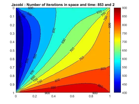
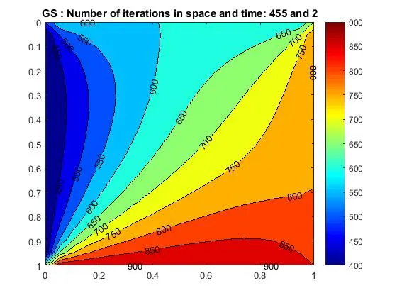
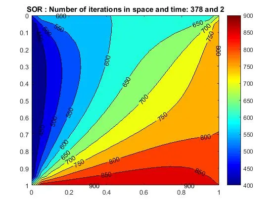
From the above plots it is clearly evident that the number of iterations are decreasing in the successive iteration.
It can be thus concluded that for number of iterations
Jacobi>Gauss Siedel>Successive over relaxation.