Week 11 - Simulation of Flow through a pipe in OpenFoam
In this challange the main objectives are-
- Write a program in Matlab that can generate the computational mesh automatically for any wedge angle and grading schemes
- For a baseline mesh, show that the velocity profile matches with the Hagen poiseuille's equation
- Show that the velocity profile is fully developed
- Post process velocity and shear stress
The main outcomes of this challange are-
1. To automate the blockMesh file such that there can be required mesh file generated at different wedge angle.
2. To calculate difference between analytical and experimental results.
This whole work is based to verify the Hagen poiseuille's equation which is discussed below-
In nonideal fluid dynamics, the Hagen–Poiseuille equation, also known as the Hagen–Poiseuille law, Poiseuille law or Poiseuille equation, is a physical law that gives the pressure drop in an incompressible and Newtonian fluid in laminar flow flowing through a long cylindrical pipe of constant cross section. Basic assumption of the equation are that fluid is incompressible and Newtonian. Poiseuille's Equation describes the pressure drop due to the viscosity of the fluid; Other types of pressure drops may still occur in a fluid.
Boundary layer
The layer in which the shearing viscous forces are significant, is called the boundary layer. This boundary layer is a hypothetical concept. It divides the flow in pipe into two regions:
- Boundary layer region: The region in which viscous effects and the velocity changes are significant.
- The irrotational (core) flow region: The region in which viscous effects and velocity changes are negligible, also known as the inviscid core.
When the fluid just enters the pipe, the thickness of the boundary layer gradually increases from zero moving in the direction of fluid flow and eventually reaches the pipe center and fills the entire pipe. This region from the entrance of pipe to the point where the boundary layer covers the entire pipe is termed as the hydrodynamic entrance region and length of the pipe in this region is termed as the hydrodynamic entry length. In this region the velocity profile develops and thus the flow is called the hydrodynamically developing flow. After this region, the velocity profile is fully developed and continues unchanged. This region is called the hydrodynamically fully developed region. But this is not the fully developed fluid flow until the normalized fluid profile also becomes constant.
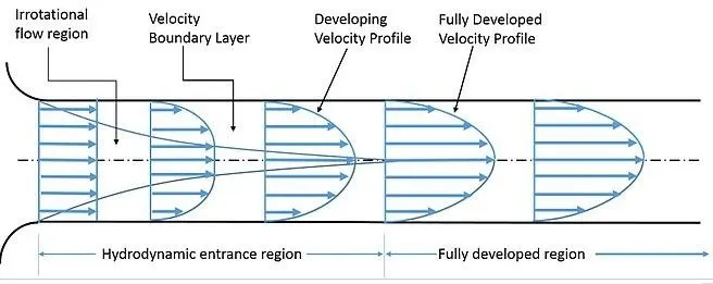
The various equations that came out of the equations are-
1. Reynolds Number: `Re = rho*V_(avg)*D//mu`
2. Velocity in fully developed region: `U = 2*V_(avg)*(1-r^2/R^2)`
3. Hydrodynamic Entrance Length: `L_e = 0.05*Re*D`
4. Pressure drop across length: `DeltaP = 32*mu*L*V_(avg)//D^2`
5. Darcy Friction: `f = 64//Re`
6. Wall Shear stress: `tau_w = (f*rho*V_(avg)^2)//8`
The basic inlet requirements are taken as:
wedge angle = 4 degrees;
Diameter of pipe = 0.02m;
Length of Piper = 2.5m;
Density of Fluid = 997 `kg//m^3`;
Dynamic Viscosity of Fluid = 0.00089 Pa*sec
The whole problem is solved using icoFoam solver in Openfoam and the Blockmesh file is made automated in Matlab such that the user can have have ease to get results at different angles.
The script file for matlab code is :
clear all
close all
clc

f1 = fopen('blockMeshDict.txt','w');

scale = 1;
theta = 4;
Re = 2100;
r = 0.01;
D=2*r;
l = 2.5;
nx = 25;
ny = 1;
nz =200;


fprintf(f1,'/*--------------------------------*-');
fprintf(f1,'C++ -*----------------------------------');
fprintf(f1,'\n');
fprintf(f1,'  =========                |\n');
fprintf(f1,'  \\      /  F ield         | OpenFOAM: The Open Source CFD Toolbox\n');
fprintf(f1,'   \\    /   O peration     | Website:  https://openfoam.org\n');
fprintf(f1,'    \\  /    A nd           | Version:  8\n');
fprintf(f1,'     \\/     M anipulation  |\n');
fprintf(f1,'---------------------------------------------------------------------------*/')
fprintf(f1,'\n');
fprintf(f1,'FoamFile\n');
fprintf(f1,'{\n');
fprintf(f1,'    version     2.0;\n');
fprintf(f1,'    format      ascii;\n');
fprintf(f1,'    class       dictionary;\n');
fprintf(f1,'    object      blockMeshDict;\n');
fprintf(f1,'}\n');
fprintf(f1,'// * * * * * * * * * * * * * * * * * * * * * * * * * * * * * * ');
fprintf(f1,'* * * * * * * //\n');
fprintf(f1,'\n');
fprintf(f1,'convertToMeters %d;\n',scale);
fprintf(f1,'\n');
fprintf(f1,'vertices\n');
fprintf(f1,'(\n');
fprintf(f1,'\t(%d %d %d)\n',0, 0, 0);
fprintf(f1,'\t(%d %d %d)\n',0,r*cosd(theta/2),r*sind(theta/2));
fprintf(f1,'\t(%d %d %d)\n',0,r*cosd(theta/2),-r*sind(theta/2));
fprintf(f1,'\t(%d %d %d)\n',l,0,0);
fprintf(f1,'\t(%d %d %d)\n',l,r*cosd(theta/2),r*sind(theta/2));
fprintf(f1,'\t(%d %d %d)\n',l,r*cosd(theta/2),-r*sind(theta/2));
fprintf(f1,');\n');
fprintf(f1,'\n');
fprintf(f1,'blocks\n');
fprintf(f1,'(\n');
fprintf(f1,'\thex (0 2 1 0 3 5 4 3) (%d %d %d) simpleGrading (1 1 1)\n',nx,ny,nz);
fprintf(f1,');\n');
fprintf(f1,'\n');
fprintf(f1,'boundary\n');
fprintf(f1,'(\n');

fprintf(f1,'    inlet\n');
fprintf(f1,'    {\n');
fprintf(f1,'        type patch;\n');
fprintf(f1,'        faces\n');
fprintf(f1,'        (\n');
fprintf(f1,'            (0 2 1 0)\n');
fprintf(f1,'        );\n');
fprintf(f1,'    }\n');

fprintf(f1,'    outlet\n');
fprintf(f1,'    {\n');
fprintf(f1,'        type patch;\n');
fprintf(f1,'        faces\n');
fprintf(f1,'        (\n');
fprintf(f1,'            (3 4 5 3)\n');
fprintf(f1,'        );\n');
fprintf(f1,'    }\n');

fprintf(f1,'    top\n');
fprintf(f1,'    {\n');
fprintf(f1,'        type wall;\n');
fprintf(f1,'        faces\n');
fprintf(f1,'        (\n');
fprintf(f1,'            (1 2 5 4)\n');
fprintf(f1,'        );\n');
fprintf(f1,'    }\n');

fprintf(f1,'    front\n');
fprintf(f1,'    {\n');
fprintf(f1,'        type wedge;\n');
fprintf(f1,'        faces\n');
fprintf(f1,'        (\n');
fprintf(f1,'            (0 1 4 3)\n');
fprintf(f1,'        );\n');
fprintf(f1,'    }\n');

fprintf(f1,'    back\n');
fprintf(f1,'    {\n');
fprintf(f1,'        type wedge;\n');
fprintf(f1,'        faces\n');
fprintf(f1,'        (\n');
fprintf(f1,'            (0 3 5 2)\n');
fprintf(f1,'        );\n');
fprintf(f1,'    }\n');

fprintf(f1,');\n');
fprintf(f1,'\n');
fprintf(f1,'mergePatchPairs\n');
fprintf(f1,'(\n');
fprintf(f1,');\n');
fprintf(f1,'\n');
fprintf(f1,'//\n');
fprintf(f1,'**************************************************************');
fprintf(f1,'*********** //\n');


fclose(f1)
The Output Blockmesh file is:
/*--------------------------------*- C++ -*----------------------------------*\
  =========                 |
  \\      /  F ield         | OpenFOAM: The Open Source CFD Toolbox
   \\    /   O peration     | Website:  https://openfoam.org
    \\  /    A nd           | Version:  8
     \\/     M anipulation  |
\*---------------------------------------------------------------------------*/
FoamFile
{
    version     2.0;
    format      ascii;
    class       dictionary;
    object      blockMeshDict;
}
// * * * * * * * * * * * * * * * * * * * * * * * * * * * * * * * * * * * * * //

convertToMeters 1;

vertices
(
	(0 0 0)
	(0 0.009994 0.000349)
	(0 0.009994 -0.000349)
	(2.5 0 0)
	(2.5 0.009994 0.000349)
	(2.5 0.009994 -0.000349)
);

blocks
(
	hex (0 2 1 0 3 5 4 3) (25 1 200) simpleGrading (1 1 1)
);

boundary
(
    inlet
    {
        type patch;
        faces
        (
            (0 2 1 0)

        );
    }
    outlet
    {
        type patch;
        faces
        (
            (3 4 5 3)

        );
    }
    top
    {
        type wall;
        faces
        (
            (1 2 5 4)

        );
    }
    front
    {
        type wedge;
        faces
        (
            (0 1 4 3)


        );
     }
    back
    {
        type wedge;
        faces
        (
            (0 3 5 2)

        );
    }

);

mergePatchPairs
(
);

//
************************************************************************* //
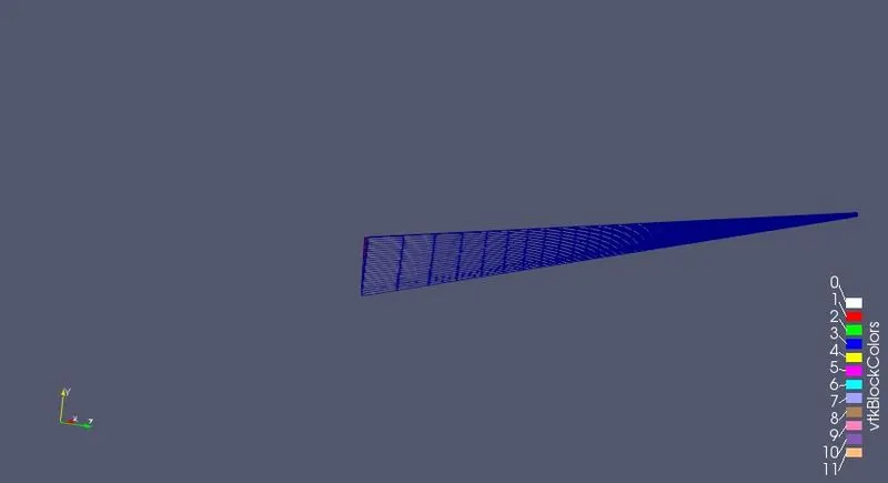
The above blockmeshDict file is run to check the mesh file and in result we get:
The Other inlet conditions like pressure and velocity and dynamic viscosity are given as:
1. Pressure:
/*--------------------------------*- C++ -*----------------------------------*\
  =========                 |
  \\      /  F ield         | OpenFOAM: The Open Source CFD Toolbox
   \\    /   O peration     | Website:  https://openfoam.org
    \\  /    A nd           | Version:  8
     \\/     M anipulation  |
\*---------------------------------------------------------------------------*/
FoamFile
{
    version     2.0;
    format      ascii;
    class       volScalarField;
    object      p;
}
// * * * * * * * * * * * * * * * * * * * * * * * * * * * * * * * * * * * * * //

dimensions      [0 2 -2 0 0 0 0];

internalField   uniform 0;

boundaryField
{
    inlet
    {
        type            zeroGradient;
    }

    outlet
    {
        type            fixedValue;
        value          uniform 0;
    }

    top
    {
        type            zeroGradient;
    }
    front
    {
        type            wedge;
    }
    back
    {
        type            wedge;
    }
}

// ************************************************************************* //
2. Velocity:
/*--------------------------------*- C++ -*----------------------------------*\
  =========                 |
  \\      /  F ield         | OpenFOAM: The Open Source CFD Toolbox
   \\    /   O peration     | Website:  https://openfoam.org
    \\  /    A nd           | Version:  8
     \\/     M anipulation  |
\*---------------------------------------------------------------------------*/
FoamFile
{
    version     2.0;
    format      ascii;
    class       volVectorField;
    object      U;
}
// * * * * * * * * * * * * * * * * * * * * * * * * * * * * * * * * * * * * * //

dimensions      [0 1 -1 0 0 0 0];

internalField   uniform (0 0 0);

boundaryField
{
    inlet
    {
        type            fixedValue;
        value           uniform (0.09373 0 0);
    }

    outlet
    {
        type            zeroGradient;
    }
    top
    {
        type            noSlip;
    }
    front
    {
        type            wedge;
    }

    back
    {
        type            wedge;
    }
}

// ************************************************************************* //
3. Transport properties:
/*--------------------------------*- C++ -*----------------------------------*\
  =========                 |
  \\      /  F ield         | OpenFOAM: The Open Source CFD Toolbox
   \\    /   O peration     | Website:  https://openfoam.org
    \\  /    A nd           | Version:  8
     \\/     M anipulation  |
\*---------------------------------------------------------------------------*/
FoamFile
{
    version     2.0;
    format      ascii;
    class       dictionary;
    location    "constant";
    object      transportProperties;
}
// * * * * * * * * * * * * * * * * * * * * * * * * * * * * * * * * * * * * * //

nu              [0 2 -1 0 0 0 0] 0.0000008927;


// ************************************************************************* //
Post processing:
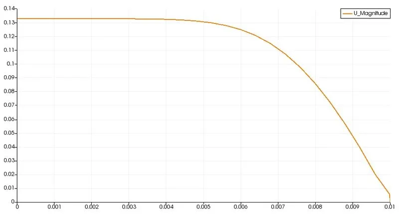
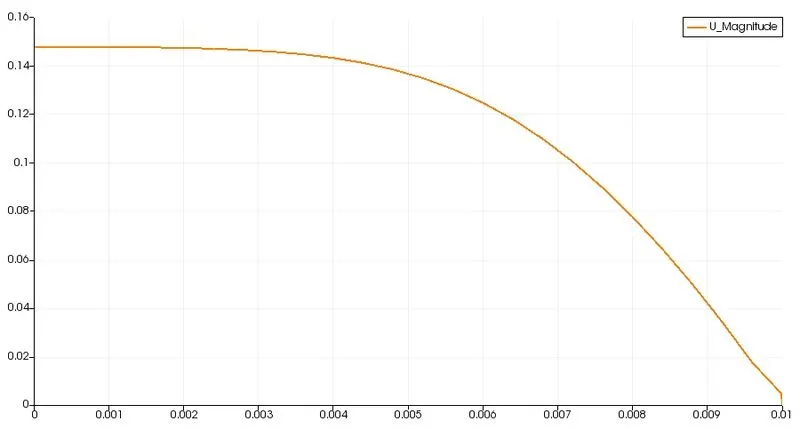
In the post processing, Varies entries were observed such as the development of velocity. It can be observed when there is rigrous velocity checking at different length of the pipe and when we get a constant output then our flow is fully developed. The velocity distribution is given as:
- At 0.2m:
- At 0.4m:
- At 0.6m:
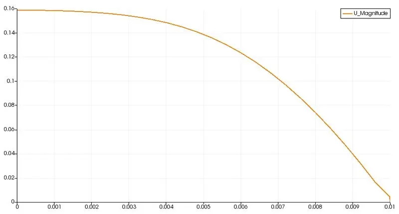
- At 0.8m:
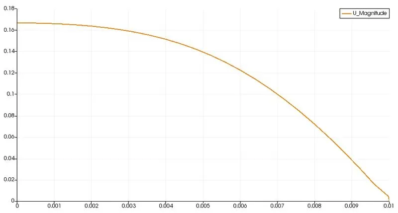
- At 1m
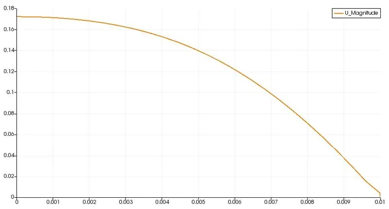
- At 1.2m:
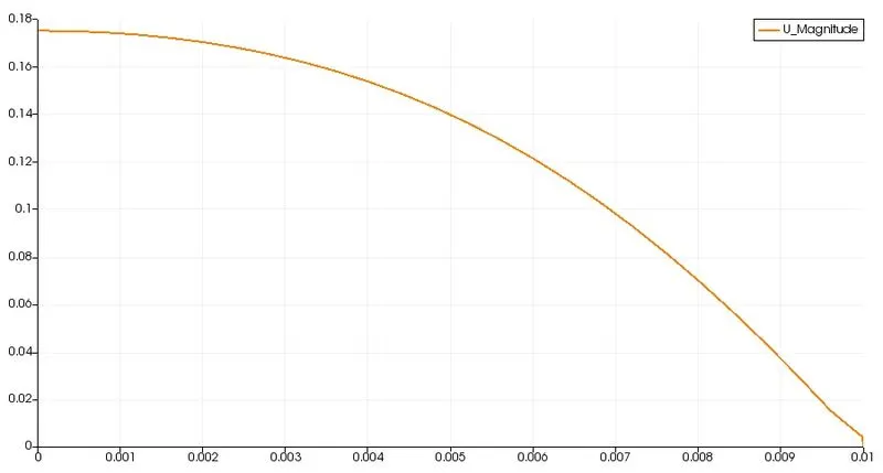
- At 1.4m:
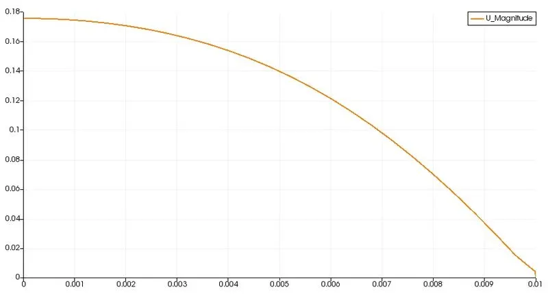
From the above plots It can be observed that the value of max velocity at center saturates after 1.2m of length.
Also It can be observe from the following plot as:
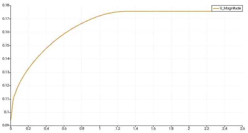
The above plot also clarifies the same about the length after which the flow gets fully developed.
Shear Stress Variation:
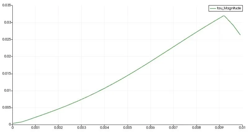
The shear stress variation in the pipe flow can also be taken out from the Openfoam and the resulting file is:
In the hydrodynamic entrance region, the wall shear stress (τw ) is highest at the pipe inlet, where the boundary layer thickness is the smallest. Shear stress decreases along the flow direction. That is why the pressure drop is highest in the entrance region of a pipe, which increases the average friction factor for the whole pipe. This increase in the friction factor is negligible for long pipes.
In fully developed region the pressure gradient and the shear stress in flow are in balance.
Comparision of Results:
| Variables | Software Results | Analytical values | Error |
| Pressure At 1.6 m | 0.00166320 pa | 0.00134 pa | 0.0003232 pa |
| Velocity At 1.6m | 0.175643 m/s^2 | 0.1855 m/s^2 | 0.00987 m/s^2 |
| Pressure Difference | 0.001534461 pa | 0.00134 pa | 0.00019446 pa |
From the above results it can be deduced that there is very minimal error in the software results and hence if this is our acceptable range then we can easily use the icoFoam solver in Openfoam to get our results for the laminar flow inside a pipe.