Week 8: Literature review - RANS derivation and analysis
In fluid dynamics, turbulence or turbulent flow is fluid motion characterized by chaotic changes in pressure and flow velocity. It is in contrast to a laminar flow, which occurs when a fluid flows in parallel layers, with no disruption between those layers.
Turbulence is commonly observed in everyday phenomena such as surf, fast flowing rivers, billowing storm clouds, or smoke from a chimney, and most fluid flows occurring in nature or created in engineering applications are turbulent. Turbulence is caused by excessive kinetic energy in parts of a fluid flow, which overcomes the damping effect of the fluid's viscosity. For this reason turbulence is commonly realized in low viscosity fluids. In general terms, in turbulent flow, unsteady vortices appear of many sizes which interact with each other, consequently drag due to friction effects increases. This increases the energy needed to pump fluid through a pipe.
REYNOLDS AVERAGED NAVIER-STOKES EQUATION`
By hand of a time-averaging of the NS equations and the continuity equation for incompressible fluids, the basic equations for the averaged turbulent flow will be derived in the following. The flow field can then be described only with help of the mean values. In order to be able to take a time-average, the momentary value is decomposed into the parts mean
value and fluctuating value. This is shown graphically in Figure below
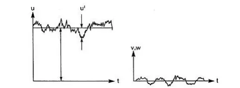
The momentary velocity components is u , the time-averaged value is named u and the fluctuating velocity has the letter u′ . With help of this definition the decomposition can mathematically be written as:
`u=overlineu+u',v=overlinev+v',w=overlinew+w'`
Governing Equations:
1. Continuity
`(partialu)/(partialx)+(partialv)/(partialy)=0`
2. Momentum
`rho((partialu)/(partialt)+u((partialu)/(partialx))+v((partialu)/(partialy)))=(-dp)/dx+mu(partial^2u)/(partialy^2)`
3. Energy
`rhoc((partialT)/(partialt)+u((partialT)/(partialx))+v((partialT)/(partialy)))=k(partial^2u)/(partialx^2)+mu((partialu)/(partialy))^2`
Reynolds Decomposition:
`u(x,y,z,t)=overlineu(x,y,z,t)+u'(x,y,z,t)`
`v(x,y,z,t)=overlinev(x,y,z,t)+v'(x,y,z,t)`
`w(x,y,z,t)=overlinew(x,y,z,t)+w'(x,y,z,t)`
Time Integration:
`overlineu(x,y)=1/(t_(INT))int_0^(t_(INT))u(x,y,z)dt`
`overlinev(x,y)=1/(t_(INT))int_0^(t_(INT))v(x,y,z)dt`
Also,
`1/(t_(INT))int_0^(t_(INT))u'(x,y,z,t)dt=0`
It is proved as following-
`u(x,y,z,t)=overlineu(x,y)+u'(x,y,z,t)`
`1/(t_(INT))int_0^(t_(INT))u(x,y,z,t)dt=1/(t_(INT))int_0^(t_(INT))u(x,y)dt+1/(t_(INT))int_0^(t_(INT))u'(x,y,z,t)dt`
`overlineu(x,y,z)=overlineu(x,y,z)+1/(t_(INT))int_0^(t_(INT))u'(x,y,z,t)dt`
`1/(t_(INT))int_0^(t_(INT))u'(x,y,z,t)dt=0`
Hence Preoved.
Now Applying Reynolds decompositon on the governing equations.
Continuity Equation
`(partialu)/(partialx)+(partialv)/(partialy)=0`
`(partial(overlineu+u'))/(partialx)+(partial(overlinev+v'))/(partialy)=0`
Integrating the above equation
`1/(t_(INT))int (partial(overlineu+u'))/(partialx)dt+ 1/(t_(INT))int (partial(overlinev+v'))/(partialy)dt=0`
`1/(t_(INT))int (partialoverlineu)/(partialx) dt+ 1/(t_(INT))int (partialu')/(partialx) dt+ 1/(t_(INT))int (partialoverlinev)/(partialy) dt+1/(t_(INT))int (partialv')/(partialy) dt=0`
SInce the flucatuating component in the above equation is zero as proved before.
Rearraging the remaining equation, we get-
`(partialoverlineu)/(partialx)+(partialoverlinev)/(partialy)=0`
Momentum Equation-
`rho((partialu)/(partialt)+u((partialu)/(partialx))+v((partialu)/(partialy)))=(-dp)/dx+mu(partial^2u)/(partialy^2)`
On rearranging-
`(partialu)/(partialt)+u((partialu)/(partialx))+v((partialu)/(partialy))=(-1)/rho*(dp)/dx+mu/rho(partial^2u)/(partialy^2)`
`(partialu)/(partialt)+u((partialu)/(partialx))+v((partialu)/(partialy))+u((partialu)/(partialx)+(partialv)/(partialy))=(-1)/rho*(dp)/dx+mu/rho(partial^2u)/(partialy^2)`
`(partialu)/(partialt)+2u((partialu)/(partialx))+v((partialu)/(partialy))+u((partialv)/(partialx))=(-1)/rho*(dp)/dx+v(partial^2u)/(partialy^2)`
Applying product rule
`(partial(uv))/(partialu)=u(partialv)/(partialy)+v(partialu)/(partialy)`
`(partialu)/(partialt)+2u(partialu)/(partialx)+(partialuv)/(partialy)=-1/rho*(partialp)/(partialx)+v((partial^2u)/(partialy^2))`
`(partialu)/(partialt)+(partialu^2)/(partialx)+(partialuv)/(partialy)=-1/rho*(partialp)/(partialx)+v((partial^2u)/(partialy^2))`
`1/(t_(INT))int_0^(t_(INT))(partial(overlineu+u'))/(partialt)dt+(partial(overlineu+u')^2)/(partialx)dt+(partial(overlineu+u')(overlinev+v'))/(partialy)dt=1/(t_(INT))int_0^(t_(INT))-1/rho*(partial(overlinep+p'))/(partialx)dt+v((partial^2(overlineu+u'))/(partialy^2)dt)`
Upon simplification-
`(partialoverlineu)/(partialt)+(partialoverline(u^2))/(partialx)+(partialoverlineuoverlinev)/(partialy)dt=-1/rho*(partialoverlinep)/(partialx)+v((partial^2u)/(partialy^2))dt-1/(t_(INT))int_0^(t_(INT))(partial(u')^2)/(partialx)dt-1/(t_(INT))int_0^(t_(INT))(partial(u'v'))/(partialx)dt`
`(partialoverlineu)/(partialt)+(partialoverline(u^2))/(partialx)+(partialoverlineuoverlinev)/(partialy)dt=-1/rho*(partialoverlinep)/(partialx)+v((partial^2u)/(partialy^2))dt-1/(t_(INT))int_0^(t_(INT))(partial(u'v'))/(partialx)dt`
`(partialoverlineu)/(partialt)+(partialoverline(u^2))/(partialx)+(partialoverlineuoverlinev)/(partialy)=-1/rho*(partialoverlinep)/(partialx)+1/rho*partial/(partialy)(mu(partialoverlineu)/(partialy)-1/(t_(INT))int_0^(t_(INT))(partial(u'v'))/(partialx)dt)`
The above equation can be physically understood as-
Inertial Term = Pressure Term + Molecular visocsity term + momentum diffusivity term (due to turbulence)
Reynold Stresses:
In fluid dynamics, the Reynolds stress is the component of the total stress tensor in a fluid obtained from the averaging operation over the Navier-Stokes equations to account for turbulent fluctuations in fluid momentum.
The geenral form of reynolds stress tensor is given as:
`tau_(ij)=-rhooverlineu_ioverlineu_j`
where `overlineu_i,overlineu_j` are the velocity direction
`x_(i or j)`is the momentum flux in the particular direction.
It is a second order tensor and is expressed as
`[[overlineu' overlineu',overlineu' overlinev',overlineu' overlinew'],[overlinev' overlineu',overlinev' overlinev', overlinev' overlinew],[overlinew' overlineu', overlinew' overlinev', overlinew' overlinew']]`
Turbulent viscosity and Molecular viscosity:
The turbulent transfer of momentum by eddies creates internal fluid friction. It is the fundamental idea of how we define viscosity in turbulent flow, i.e. internal fluid resistance. Eddy viscosity explains what causes internal friction.
Molecular viscosity is the same as viscosity. The Coefficient of Molecular Viscosity is the same value as dynamic viscosity. Molecular viscosity is the transport of mass motion momentum solely by the random motions of individual molecules not moving together in coherent groups. Molecular viscosity is analogous in laminar flow to eddy viscosity in a turbulent flow
Conclusion:
RANS is a closure loop problem which is used to estimate the time average of the required quantities inspite of solving the Navier-Stokes Equation completely over whole domain.
The selection of tubulence model depends upin the application and the type of analysis i.e. Internal flow analysis, External Flow Analysis, IC Engine problem etc.
References:
http://daad.wb.tu-harburg.de/fileadmin/BackUsersResources/Flood_Probability/2D/Steffi-2D/pdf/Reynolds_average_Navier-Stokes_equation.pdf