Week 1: Channel flow simulation using CONVERGE CFD

AIM

1. For this challenge, we will be setting up a channel flow tutorial.

2. Once you have the base setup ready, run the case for three different base mesh sizes.

3 different base mesh sizes are,

• dx = 0.001m, dy = 0.001m, dz = 0.001m
• dx = 0.0005m, dy = 0.0005m, dz = 0.0005m
• dx = 0.0004m, dy = 0.0004m, dz = 0.0004m

To show

1. Velocity and pressure contours for all the 3 base mesh sizes

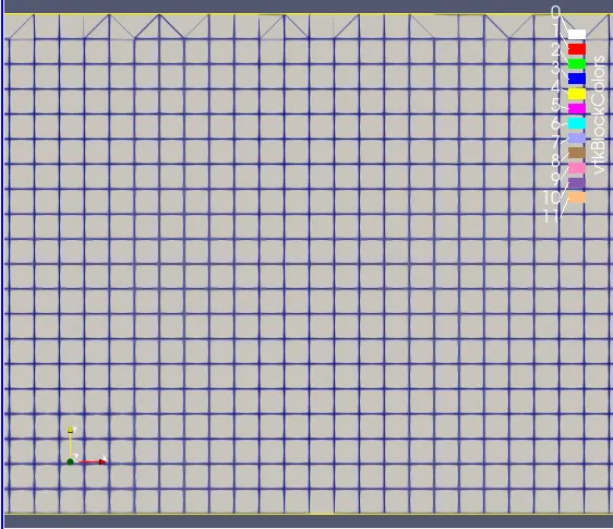
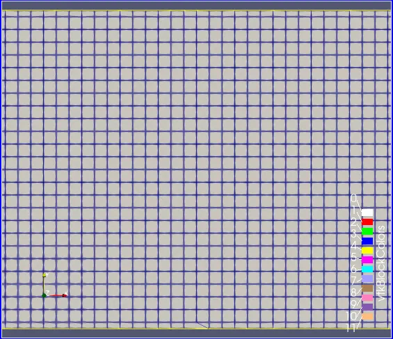
2. Show mesh (i.e surface with edges) for the 3 base mesh sizes

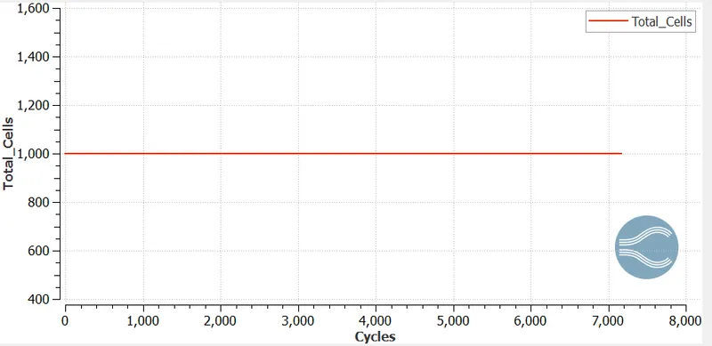
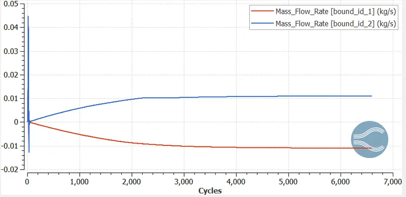
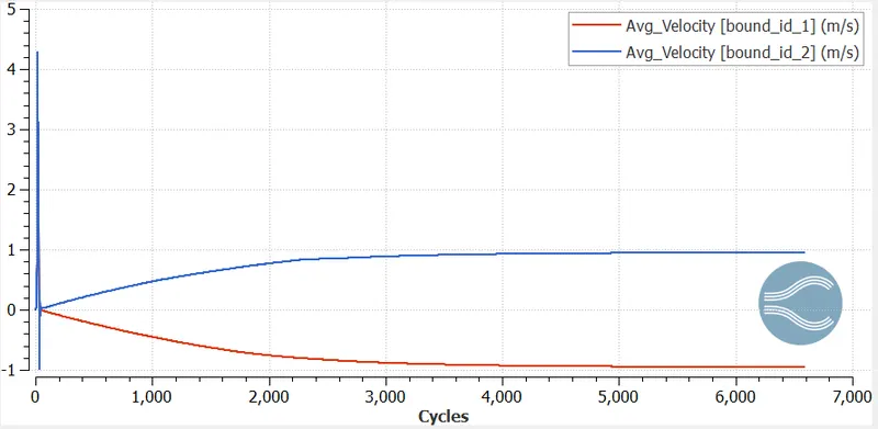
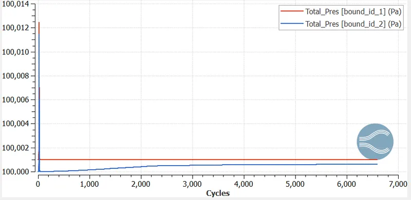
3. Plots for velocity, pressure, mass flow rate, and total cell count for all 3 base mesh sizes.

Channel flow is defined as the problem in which the fluid is flowing in a closed body (here it is a rectangular body). Since in this current study no slip condition is applied at the top and bottom walls, so a parabolic velocity profile is expected to be generated in the domain. Also, in this problem steady state case is considered and no turbulence generation is taken into account such that there is no use of turbulence models.

Modelling the problem in Converge Software

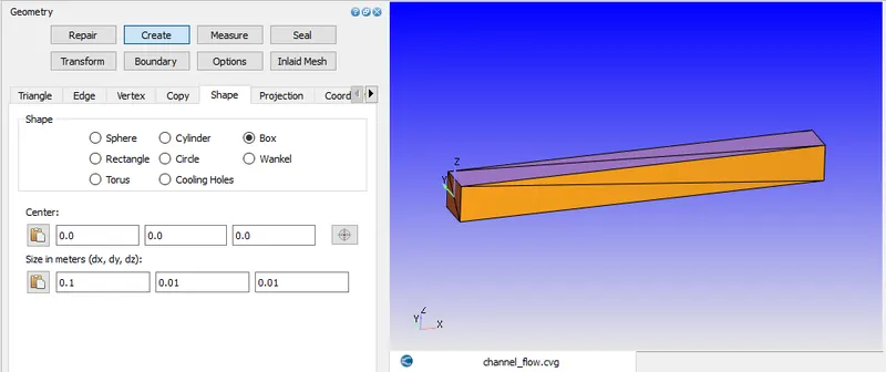
A box of the dimensions as shown in the image below is made initially

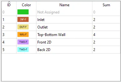
Each of the face is given a boundary name and allotted a ID.

After this normal orientation is checked and then changed to the normal pointing inward to the body.

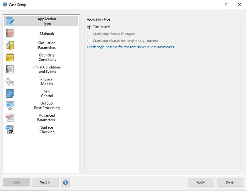
Since this is a steady state problem, the procedure to setup it is shown in the steps below.

In the materials tab "Air" is selected and species tab is checked.

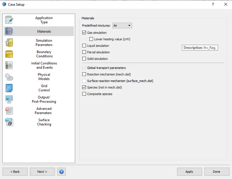
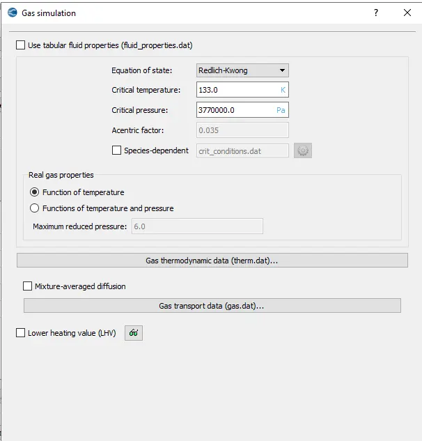
In the Gas simulation tab, default settings are set

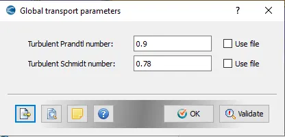
In the Global transport Parameters, defaults are kept to be same.

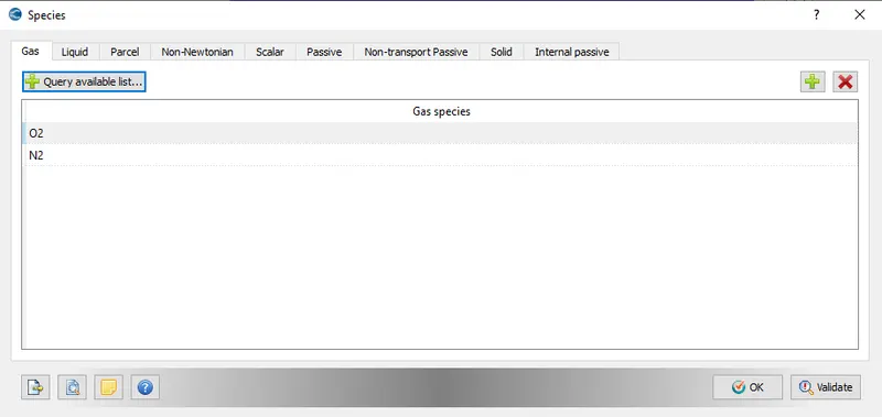
Oxygen and Nitrogen species are added in the species tab.

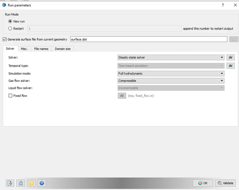
In the Run parameters tab, steady state solver is selected along with simulation mode to be in full hydrodynamic and solver used to be compressible.

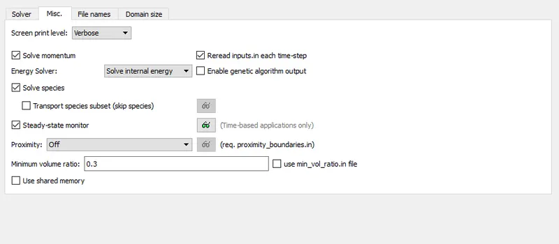
Also in the misc tab, steady state monitor is turned on for the convergence of results and shared memory tab is made off.

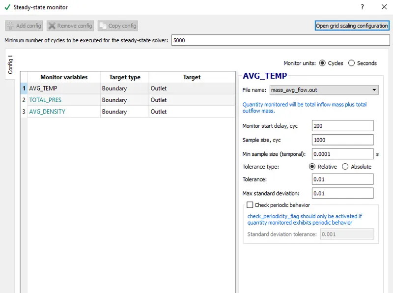
Different monitor variables are selected.

The minimum number of cycles to be executed for steady state solver are set at 5000.

monitor start delay and sample size are set at 200 and 1000 respectively, as shown below.

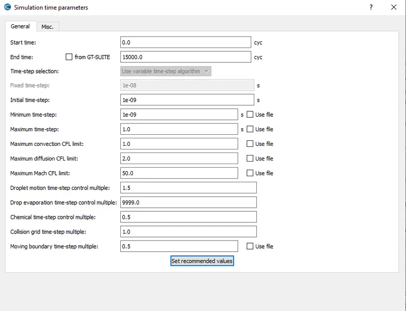
In the time parameters tab, end time is set to be at 15000 cycles and initial, minimum time steps to be 1e-09 and maximum time step is set at 1s.

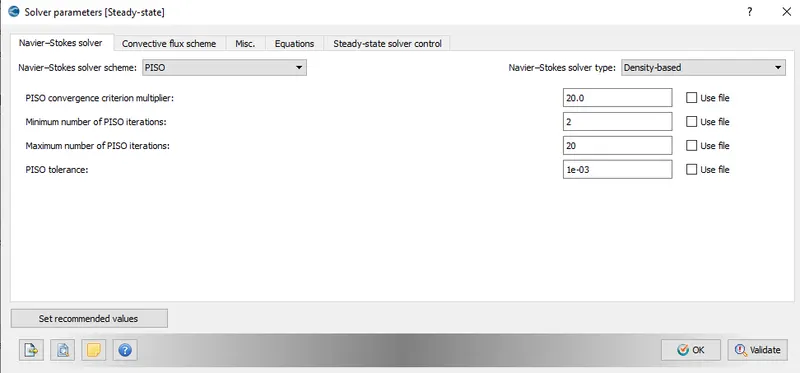
PISO scheme is selected for solving the navier stokes equation and other values are set to be at the default.

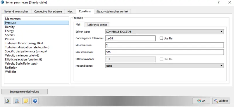
In these parameters, pressure term's precondition is set to be none.

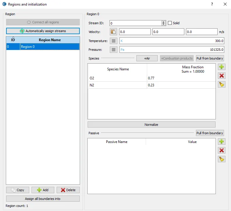
For initialization, a zone of different gases with unity summation of mass fractions and arbitrary values is set.

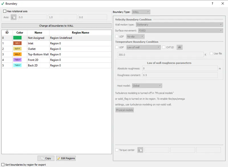
Futher the type of boundary and zone is set to all. Top and bottom faces are given a no slip condition, While others are defined the conditions as name states.

Grid sizing:

3 different size of grid are selected which are.

Mesh.no.	dx	dy	dz
1.	0.001	0.001	0.001
2.	0.0005	0.0005	0.0005
3.	0.0004	0.0004	0.0004

Mesh 1-

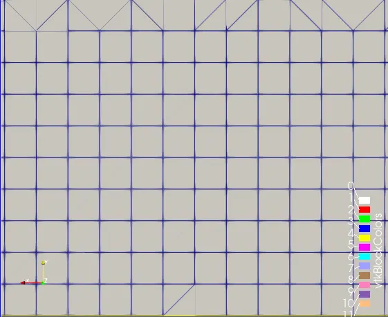
Mesh 2-

Mesh 3-

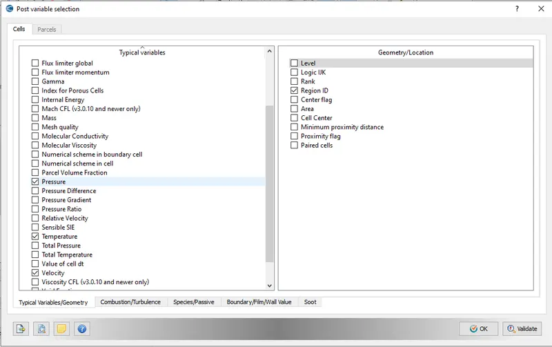
For getting the output values the required entities are selected.

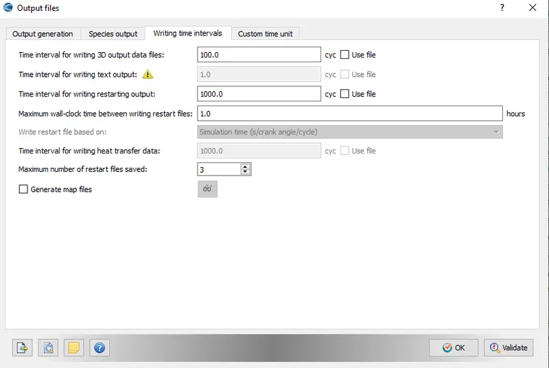
Number of cycles for 3d output data is set to be 100 cycles.

Finally the data files are exported which are solved by using the solver.

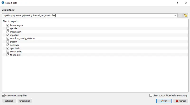
Output:

Mesh 1

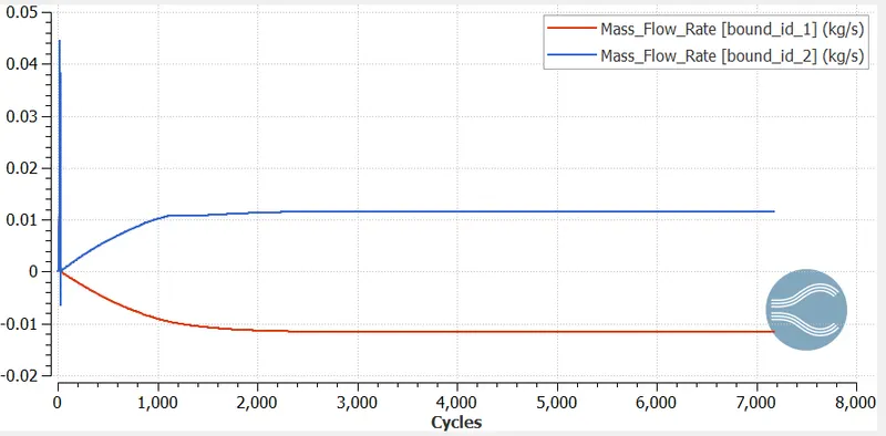
Mass Flow Rate plot at Inlet and Outlet-

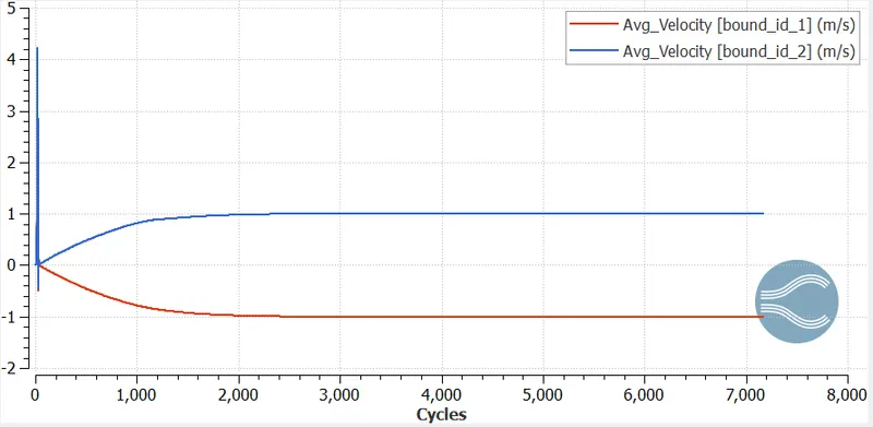
Average velocity plot at Inlet and Outlet-

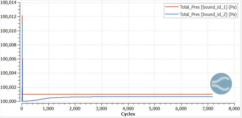
Total pressure plot at Inlet and Outlet-

Number of cells plot at Inlet and Outlet-

Velocity animation for coarse mesh-

Pressure animation for coarse mesh-

Mesh 2

Mass Flow Rate plot at Inlet and Outlet-

Average velocity plot at Inlet and Outlet-

Total pressure plot at Inlet and Outlet-

Number of cells plot at Inlet and Outlet-

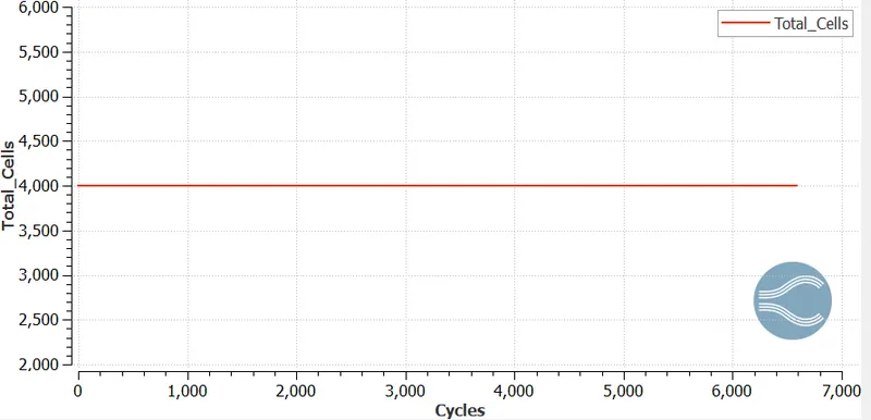
Velocity animation for coarse mesh-

Pressure animation for coarse mesh-

Mesh 3

Mass Flow Rate plot at Inlet and Outlet-

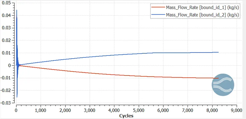
Average velocity plot at Inlet and Outlet-

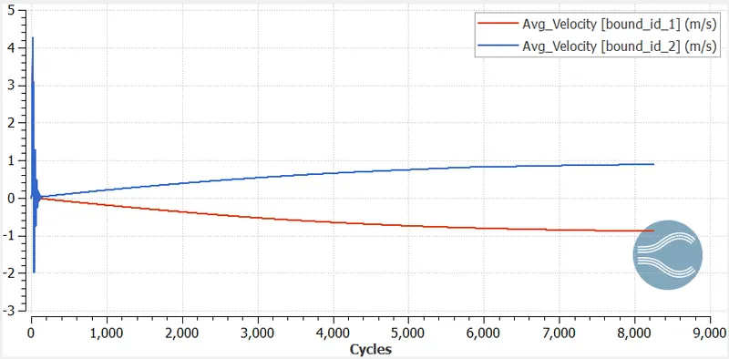
Total pressure plot at Inlet and Outlet-

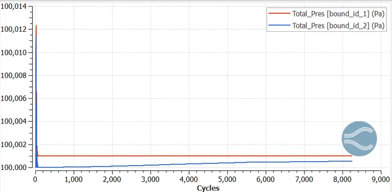
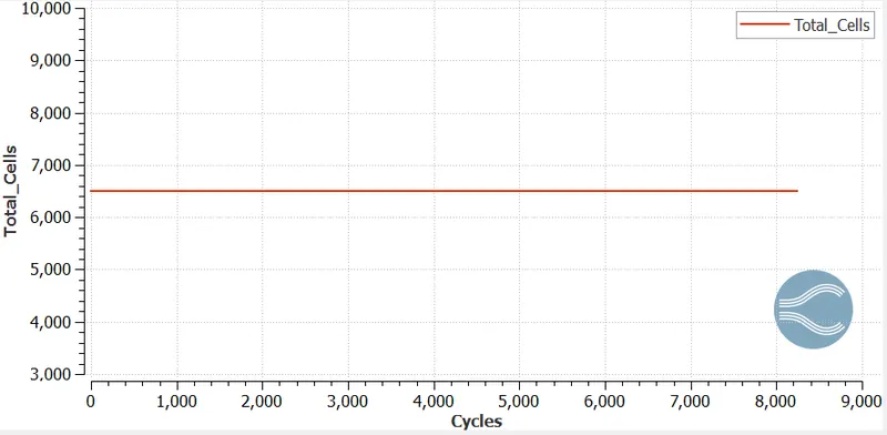
Number of cells plot at Inlet and Outlet-

Velocity animation for coarse mesh-

Pressure animation for coarse mesh-

Conclusions:

1. As we move towards the mesh refined the load on the computational power is substantially increased.
2. As the mesh size is reduced the convergence of the problem is seen to be achieved at lesser iterations.
3. The value of the velocity at each cross section seems to be near the actual results and more refined.
4. Mesh refinement increases load along with the accuracy of the results.