Week 9 - FVM Literature Review
The finite volume method (FVM) is a discretization technique for partial differential equations, especially those that arise from physical conservation laws. FVM uses a volume integral formulation of the problem with a finite partitioning set of volumes to discretize the equations. FVM is in common use for discretizing computational fluid dynamics equations.
FVM discretization and Solution Procedure:
1. The fluid domain is divided into a finite number of control volumes (cells of a computational grid).
2. Integral form of the conservation equations are discretized and applied to each of the cells.
3. The objective is to obtain a set of linear algebraic equations, where the total number of unknowns in each equation system is equal to the number of cells.
4. Solve the equation system with an solution algorithm with proper equation solvers.
Differences between FDM & FVM
FDM:
FDM is similar to differential calculus but it has killed the heart that is limit tend a to "zero". So in most of the cases accuracy of FDM increases with refining grid. Easy method but not reliable for conservative ifferential equations and solutions having shocks. Tough to implement in complex geometry where it needs complex mapping and mapping makes governing equation even tougher. Extending to higher order accuracy is very simple.
FVM:
This is similar to FDM but. It didn't kill the theme of differentiation because we are integrating the differential equation over a control volume and discretizing the domain. Since we have integrated the differential equation discetization is mathematically a valid one. Here fluxes are integrated and resultant is set to zero, so flux is conserved. Can handle almost any PDEs and complex domain. Interpolation is done from face to centre will reduce the accuracy of this process. Here accuracy is based on order of polynomial used. FVM can also produce any order accurate numerical solution similar to FDM but more
Need for Interpolation Scheme:
The 1D Steady State Heat Conduction Problem is employed for the explanation.
`dT//dx(k*dT//dx) + S = 0`
The whole control volume is divided as:
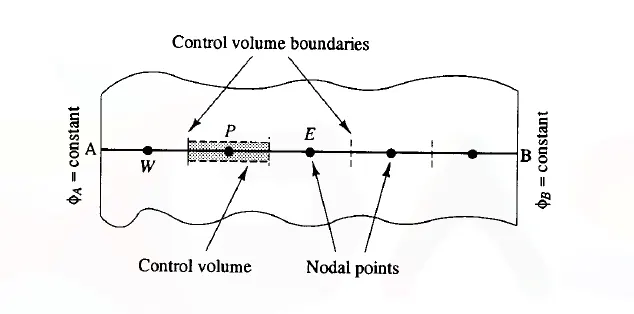
The concentrated area P is our area of focus and there are 2 neighbouring elemnets to it named west(W) and east(E). The further division is explained in the image below:
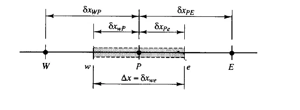
Further the above heat equation is discretized as -
`intd/dx(k*dT//dx)*dV + intS*DeltaV =0`
`(K*A*dphi//dx)_e - (K*A*dphi//dx)_w + S*DeltaV = 0`
in the above equation the value of K can be observed as-
`K_w = K_W + K_P//2`
`K_e = K_P+ K_E//2`
The diffusive flux terms can further be expanded as difference of two and the source term S can also be a dependent function. So rewriting the equation we get-
`K_e**A_e*(T_E-T_P//deltax_(PE)) - K_w**A_w*(T_P-T_W//deltax_(WP)) + (S_w + S_p*phi_p) = 0`
Further,
`(T_e/(deltax_(PE)) * A_e + T_w/(deltax_(WP)) * A_w - S_p)*phi_P = (T_e/(deltax_(PE)) * A_e )*phi_E + (T_w/(deltax_(WP)) * A_w - S_p)*phi_E +S_w`
we can reduce the above equation as-
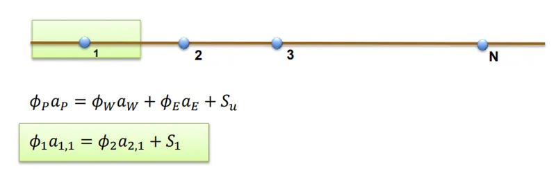
`a_P*phi_P = a_W*phi_W +a_E*phi_E +S_w`..
The above equation can solved simultaneoulsy at the nodal points by interpolating technique as to get the result at the next node we need the data at the previous one and thus it generates the value at next node. The interpolating scheme is well discussed in the following figure.
Discretization Schemes:
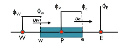
1. First Order Upwind Scheme:
We define two faces, e and w. To obtain flux through faces e and w, we need to look its neighbouring values at P/E and W/P respectively. The subscripts denote the face at which the face value or the flux F is located at.
`phi_e = phi_p` or `phi_e = phi_E`
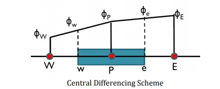
2. Central Differencing Scheme:
`phi_e = (phi_E + phi_P)/2`
`phi_w = (phi_P + phi_W)/2`
3.QUICK
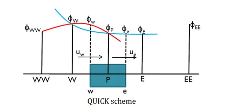
QUICK stands for Quadratic Upwind Interpolation for Convective Kinetics. In the QUICK scheme 3 point upstream-weighted quadratic interpolation are used for cell face values.