Week 7: Shock tube simulation project

Shock tube is one of the simple laboratory apparatus that can generate various flow speeds at different flow regimes. The shock tube performance is based entirely upon the pressure ratio and speed of sound in driver and driven section. The strength of shock increases in the ratio of speed of sound. Considering a shock tube where, the shock wave is generated by rupturing thin diaphragms instantly with appropriate pressure ratios across the driver and driven section of the shock tube. The pressure rises across the across primary and reflected shock is measured by high frequency pressure transducers located towards end of driven section. All necessary shock tube parameters are calculated through one- dimensional shock tube relations and are validated with experimental data.

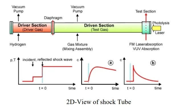
When a wave moves faster than the local speed of sound in a fluid, it is a shock wave. Like an ordinary wave, a shock wave carries energy and can propagate through a medium; however, it is characterized by an abrupt, nearly discontinuous change in pressure, temperature and density of the medium. Thus, the sonic boom associated with the passage of a supersonic aircraft is a type of sound wave produced by constructive interference.

Modelling the problem in Converge Software

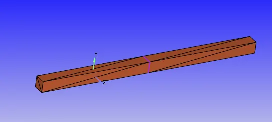
The 3D model is imported in the software.

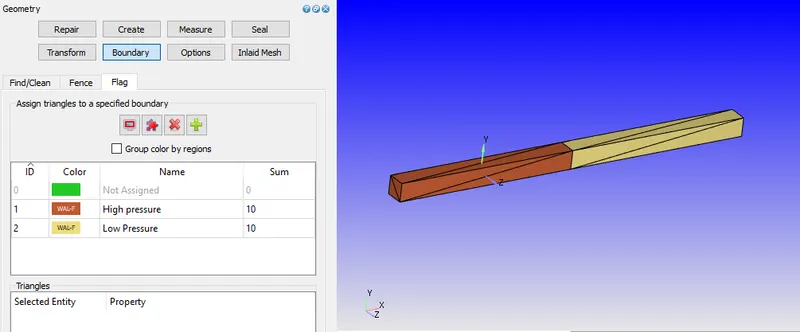
Each of the face is given a boundary name and allotted an ID.

Since this is a Transient problem, the procedure to setup it is shown in the steps below.

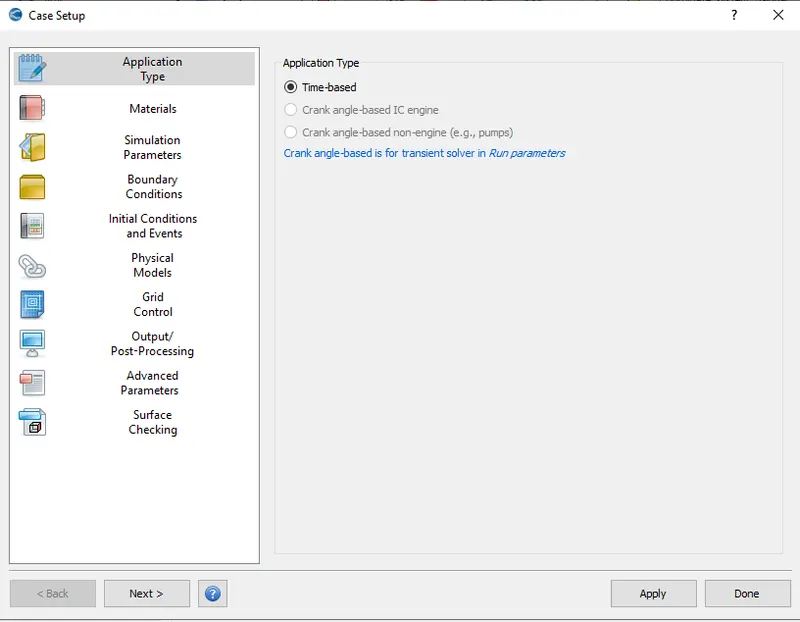
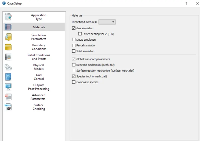
In the materials tab "Air" is selected and species tab is checked.

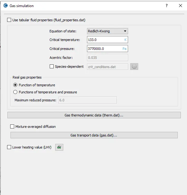
In the Gas simulation tab, default settings are set

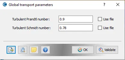
In the Global transport Parameters, defaults are kept to be same.

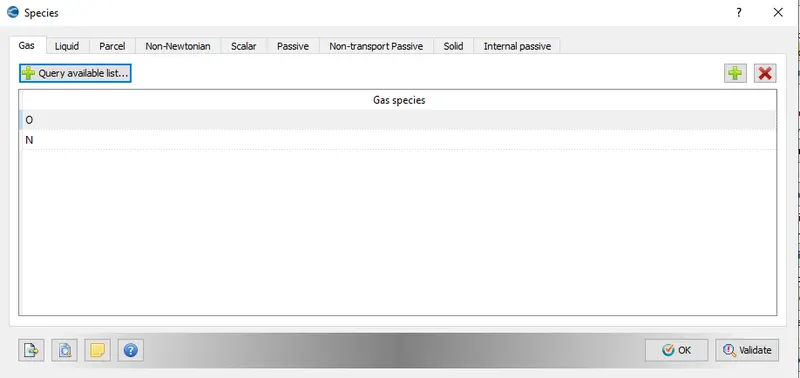
In Species tab, O and N are added

In the Run parameters tab, steady state solver is selected along with simulation mode to be in full hydrodynamic and solver used to be compressible.

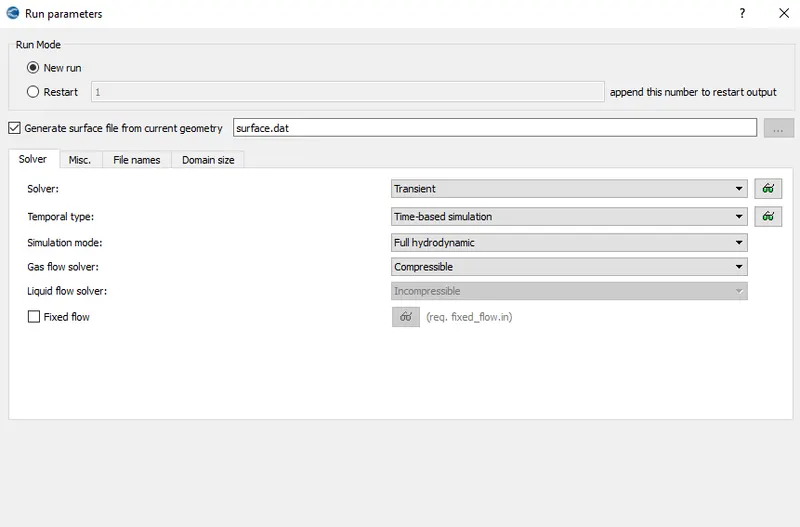
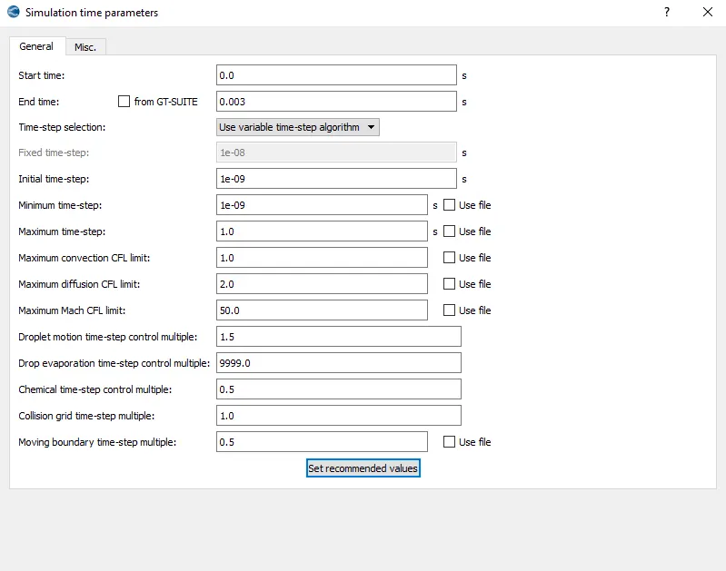
Simulation is run for 3 ms and the inputs are shown below-

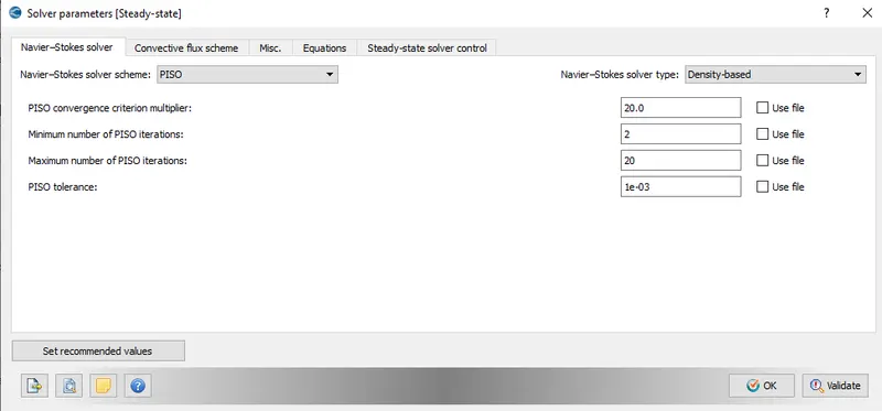
PISO scheme is selected for solving the navier stokes equation and other values are set to be at the default.

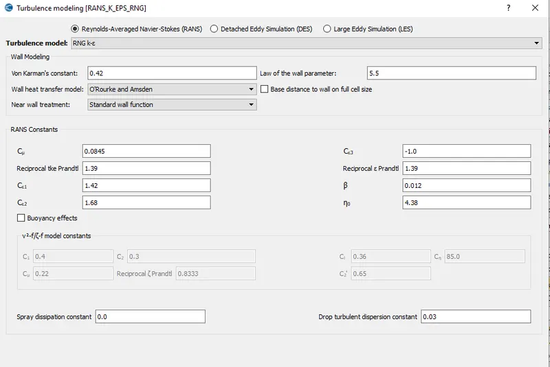
For the turbulence modelling RNGk-ε model is chosen with default values.

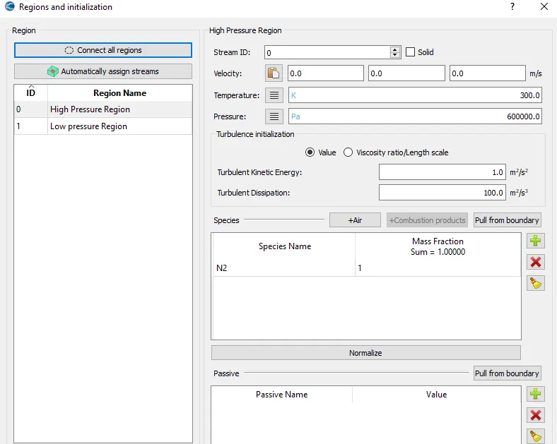
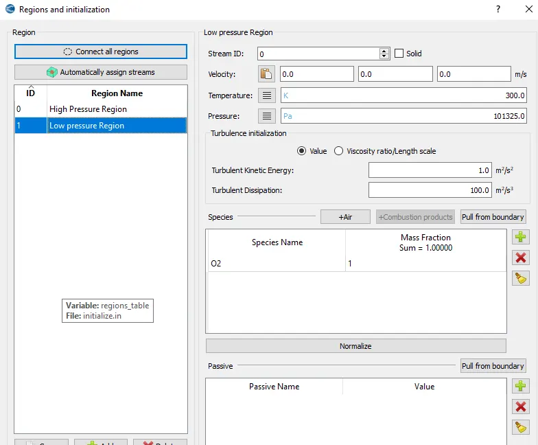
For initialization, Two different zones with high and low pressure are set,

High pressure region-

Low Pressure region-

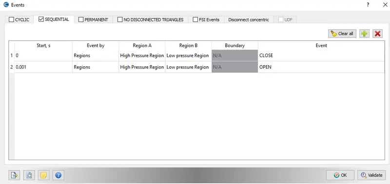
For the shock phenomenon to happen a imaginary diapgragm is put in between the two regions and its rupture time is given in the form of events as-

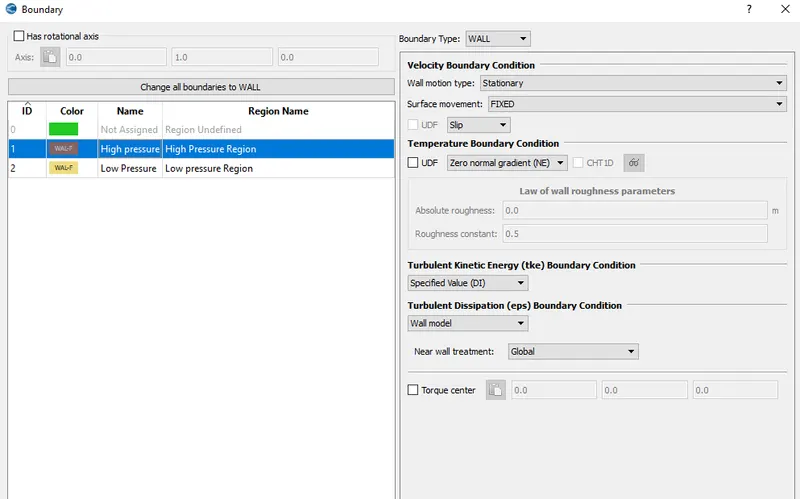
Futher the type of boundary and zone is set to all. Both of the domains are given wall boundary with slip boundary condition

Grid sizing:

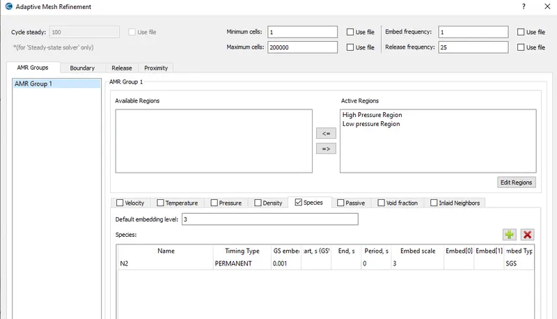
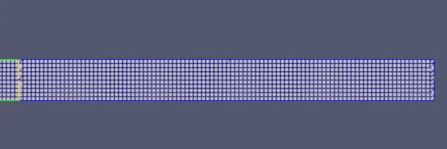
Grid of size 0.001 m is applied in all directions. Adaptive mesh refinement is applied with sub-grid criterion.

Mesh-

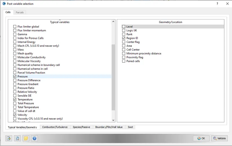
For getting the output values the required entities are selected.

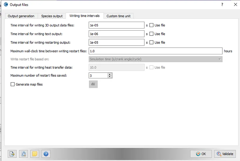
Number of cycles for 3d output data is set to be 100 cycles.

Finally the data files are exported which are solved by using the solver.

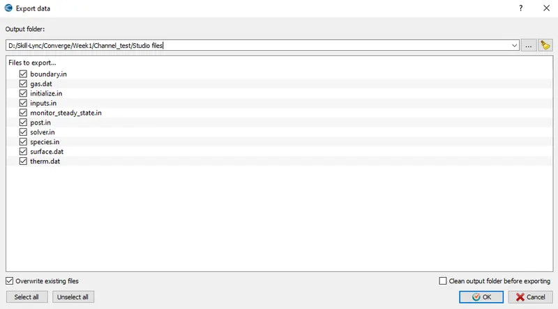
The input files are solved by using the cygwin.

Output:

Mesh animation:

Pressure contour:

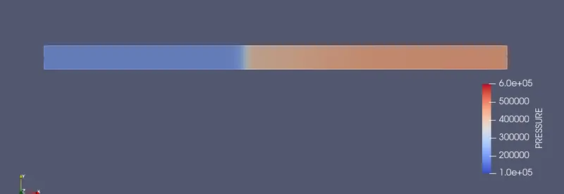
Pressure animation:

Velocity Contour:

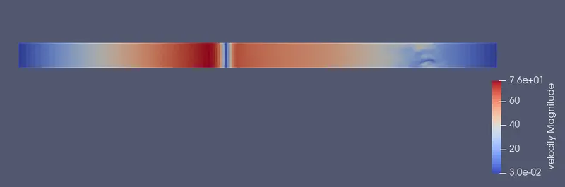
Velocity Animation:

Plot for number of cells:

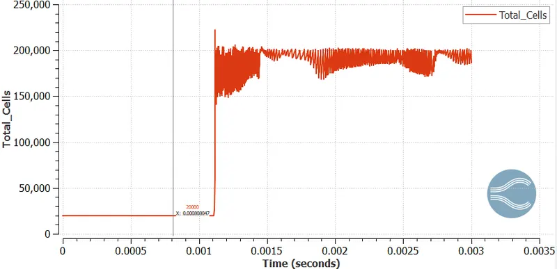
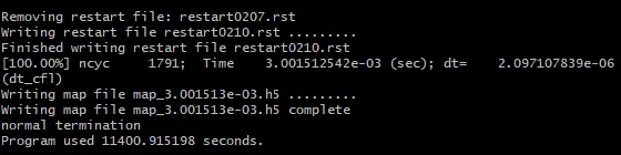
Simulation Time:

Conclusions:

1. Converge CFD Software is able to predict the shock wave phenomenon in better way.
2. The Adaptive mesh Refinement helps in better solving for the crticial areas during the simulation.
3. Mixing is observed abruptly after diaphragm removal which results in the generation of shock wave and ultimately leads to pressure and velocity fluctuations.
4. The mesh starts to change as soon as the the diaphragm is removed and it can be observed in the animation also.