Week 6: Conjugate Heat Transfer Simulation
Modelling the problem in Converge Software
Two enclosed cylinders of radius 0.015m and 0.02m are made by using te create command.
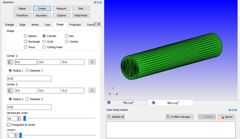
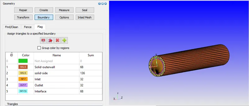
Each part is given a boundary names which is used for boundary definintion.
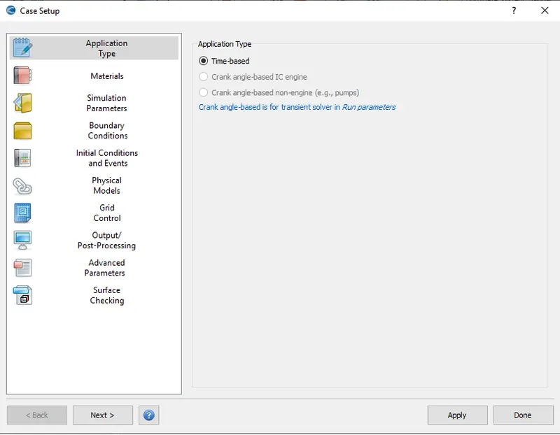
Since this is a Transient problem, the procedure to setup it is shown in the steps below.
In the materials tab "Air" is selected and species tab is checked. Since it also includes solid parts so solid smulation is also turned on.
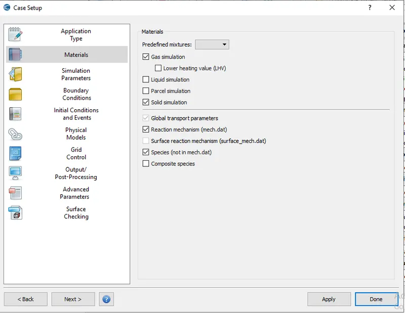
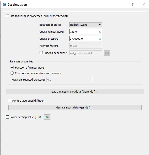
In the Gas simulation tab, default settings are set
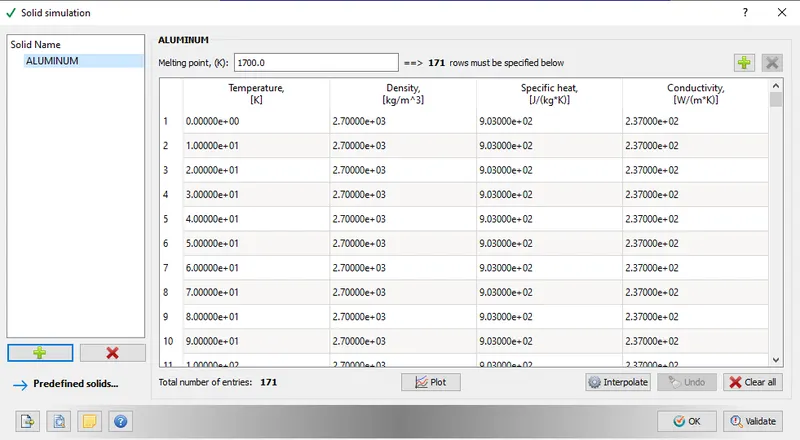
In solid simulation aluminium material is selected
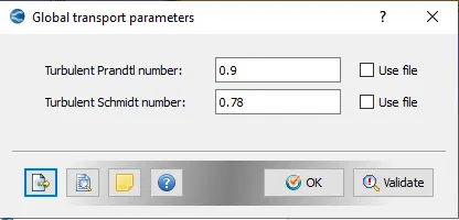
In the Global transport Parameters, defaults are kept to be same.
O and N are selected in the species tab.
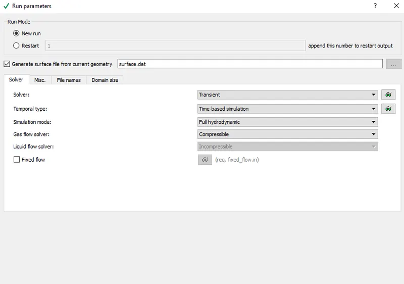
In the Run parameters tab, Transient solver is selected along with simulation mode to be in full hydrodynamic and solver used to be compressible.
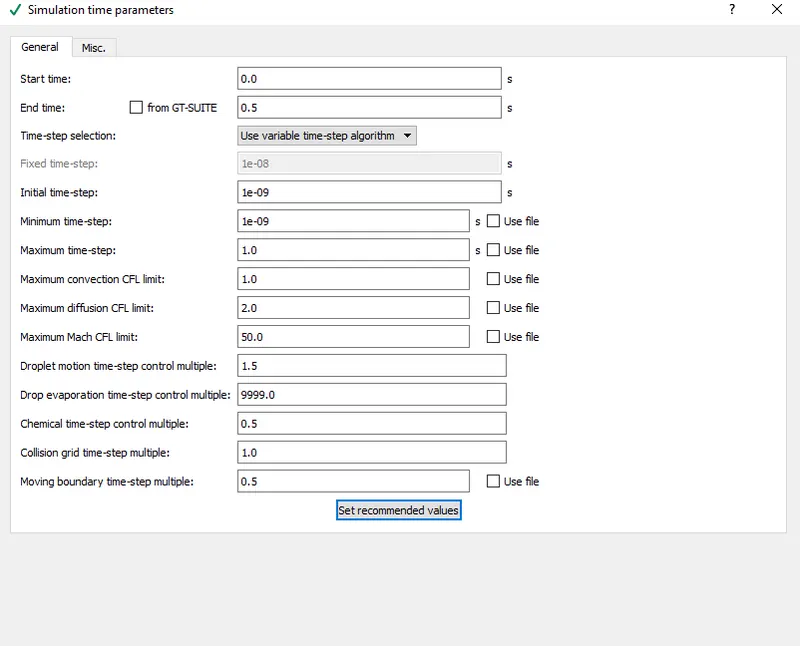
In simulation time parameters, end time is kept to be 0.5sec.
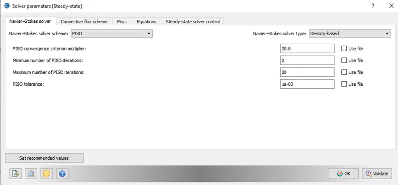
PISO scheme is selected for solving the navier stokes equation and other values are set to be at the default.
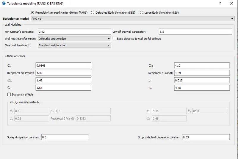
For the turbulence modelling RNG k-ε model is chosen with default values.
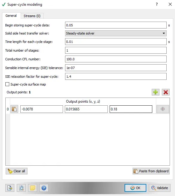
Super-cycling module is selcted and its values are entitled below-
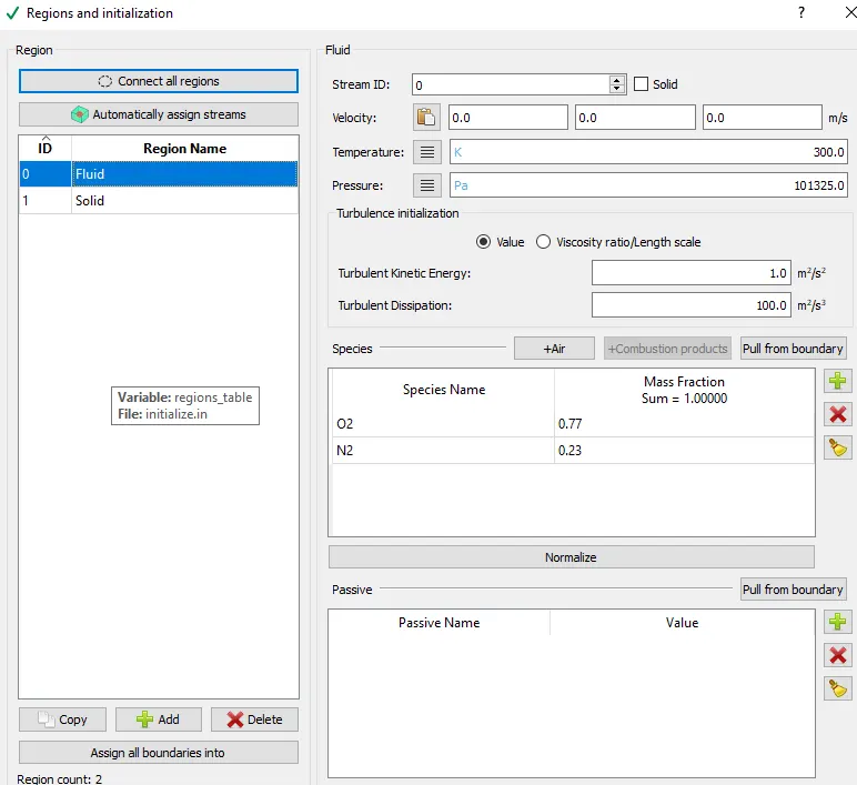
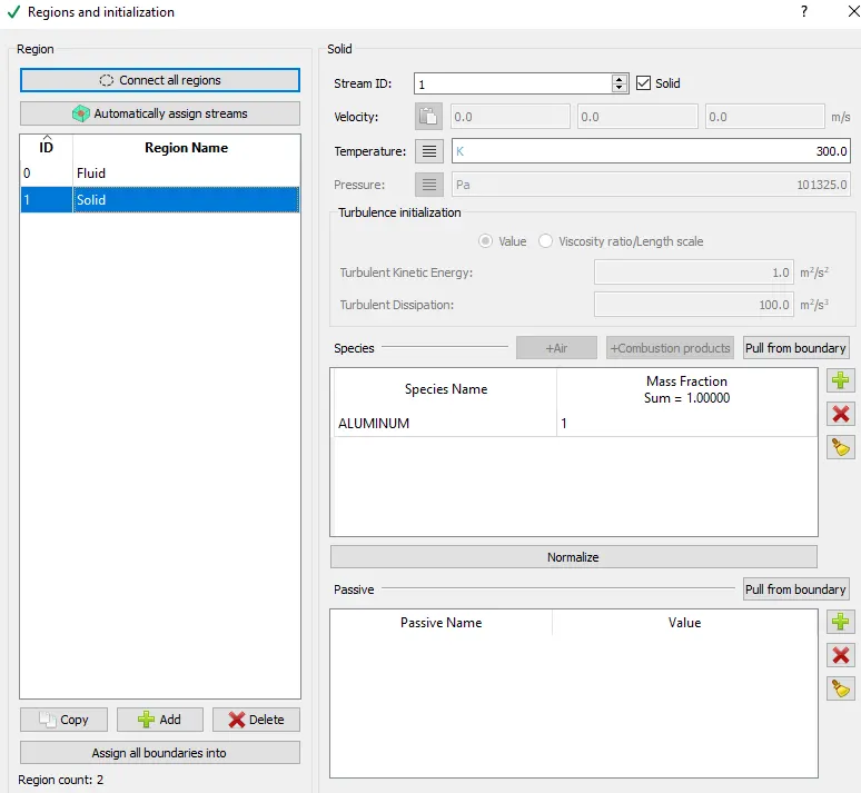
For initialization, There are two different domains i.e. Solid and Fluid, both of these are given the requied input values.
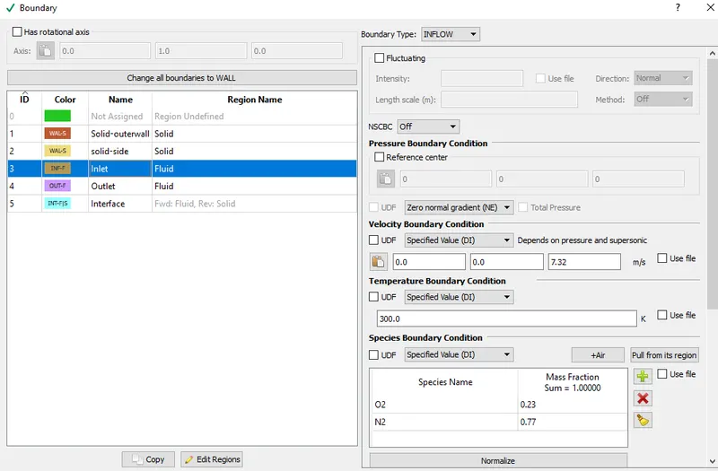
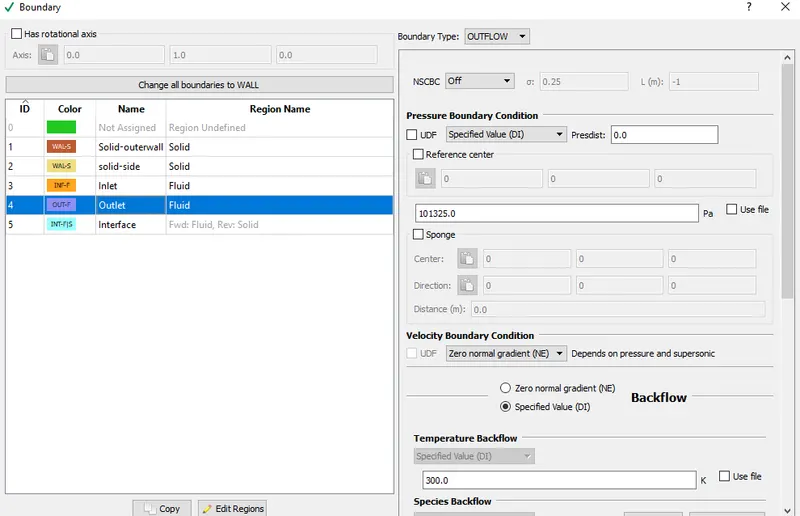
Futher the type of boundary and zone is set to all. Side walls and front and back are solid walls. Inlet and outlet are in the fluid regions. the velocity inlet for Reynolds number 7000 is defined. The interafce is applied n the inner side of the pipe which acts as interface between the two phases.
Solid outer wall is given a constant flux
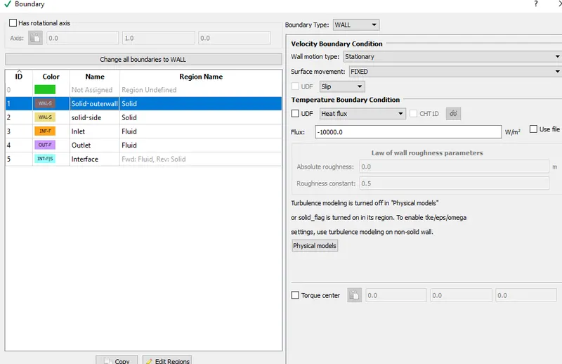
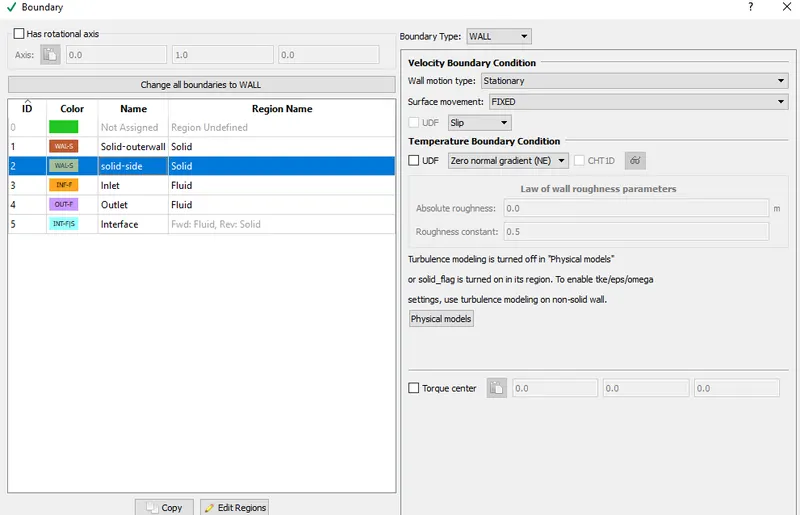
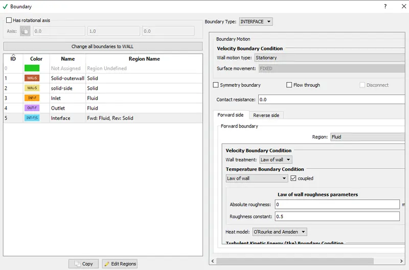
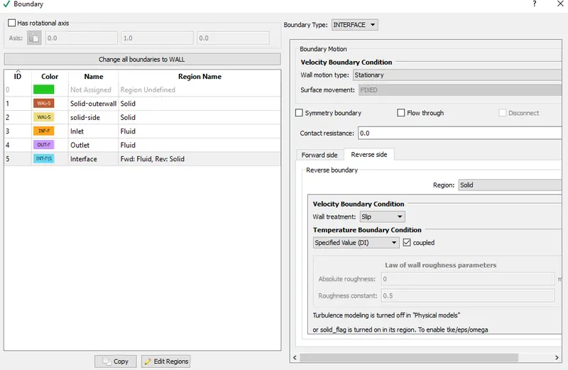
The forward side of the interafce is facing towards the fluid side and Reaer is towards solid.
Grid sizing:
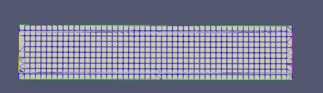
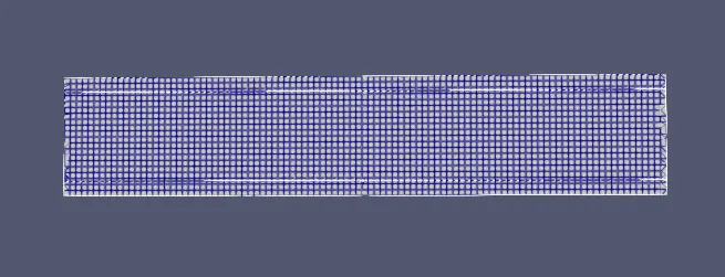
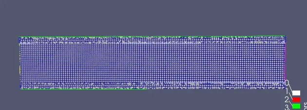
Three different mesh is applied initially.
| Mesh.no. | dx-dy-dz |
| 1. | 0.004 |
| 2. | 0.002 |
| 3. | 0.001 |
Mesh 1-
Mesh 2-
Mesh 3-
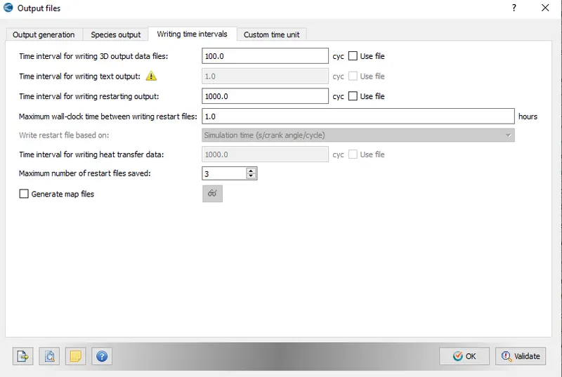
For getting the output values the required entities are selected.
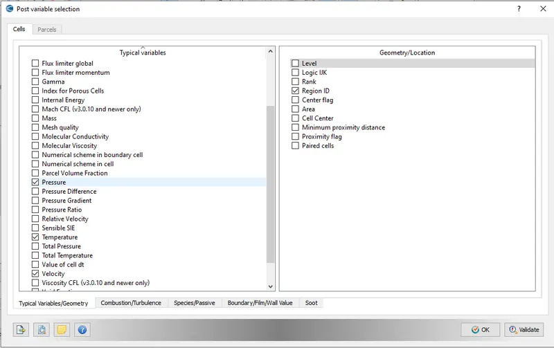
Number of cycles for 3d output data is set to be 100 cycles.
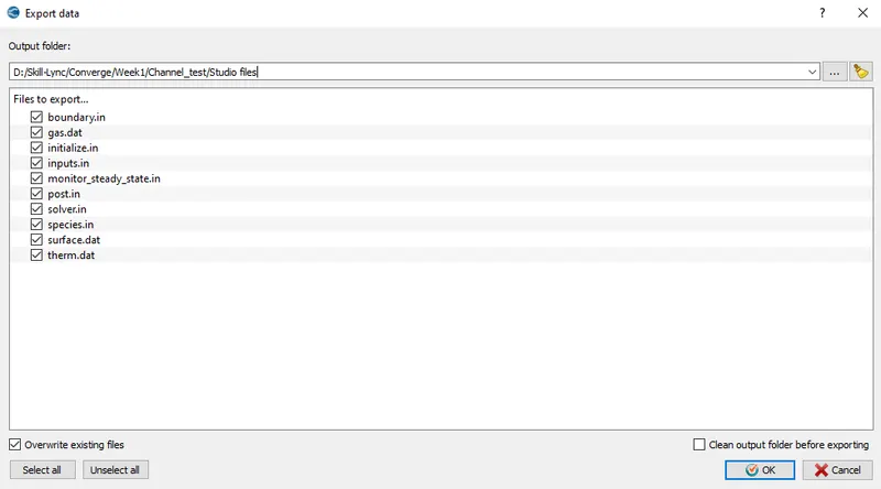
Finally the data files are exported which are solved by using the solver.
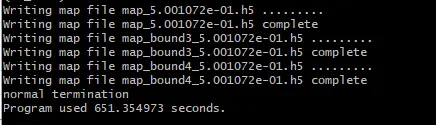
The input files are solved by using the cygwin.
Output:
Mesh 1
Completion Time:
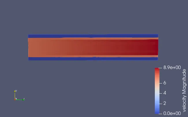
Velocity Contour:
Temperatue Contour:
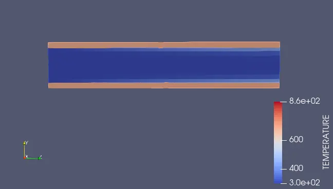
Final Temperature plot:
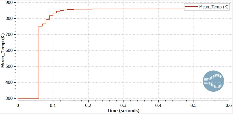
Final Temperature = 858.346K
Mesh 2
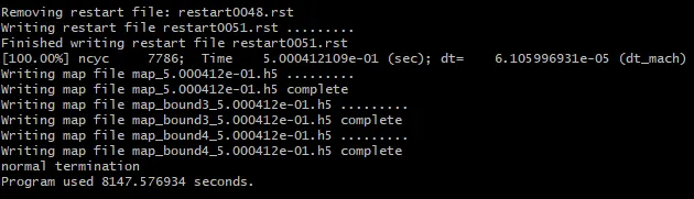
Completion Time:
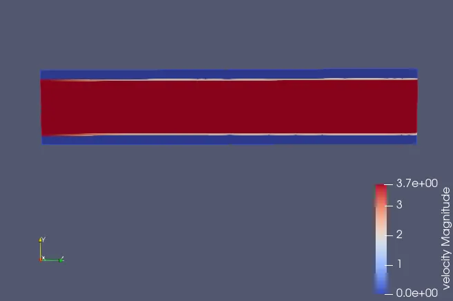
Velocity Contour:
Temperature Contour:
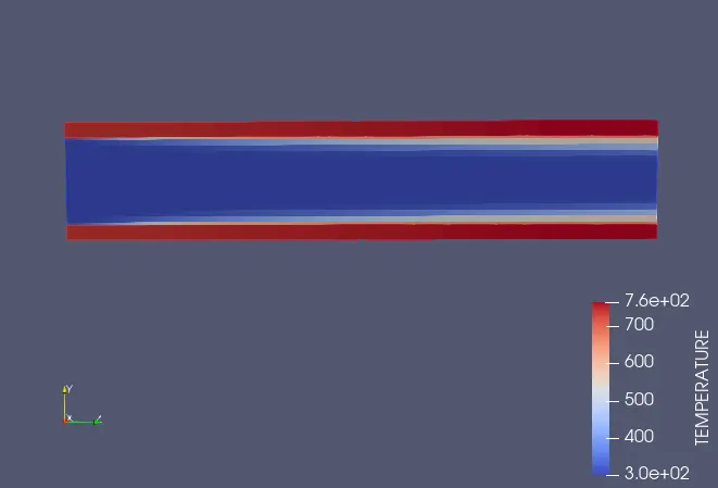
Final Temperature plot:
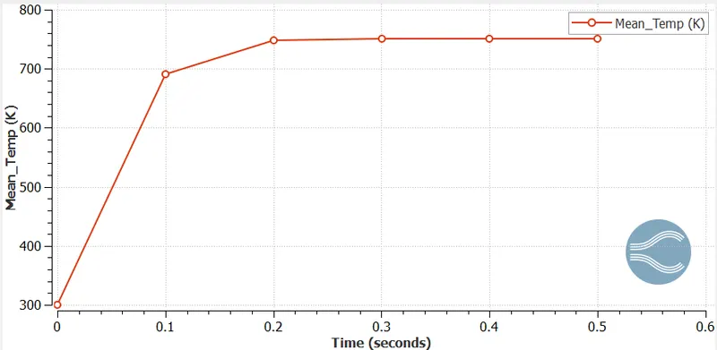
Final Temperature = K
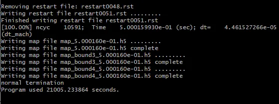
Mesh 3
Completion Time:
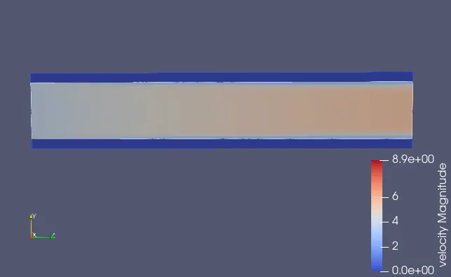
Velocity Contour:
Temperature Contour:
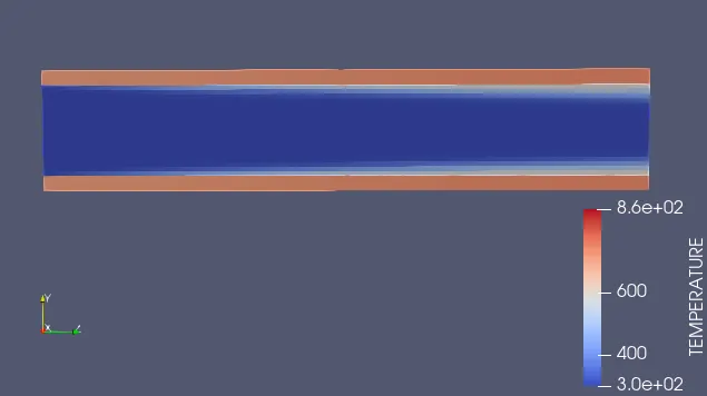
Final Temperature plot:
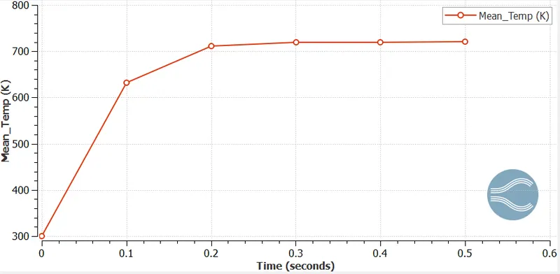
Final Temperature = 720.161K
Conclusion:
- It can be observed that with the increse in mesh count the solution approaches to more actual result.
- Supercycling helps in better prediction of temperature growth in the solid material also.
- The simulation time is directly proportional with the mesh count.
- Velocity of fluid is maximum in the centre of cylinder.
The supercyle stage interval is set to three different values for the Mesh 1 to 0.01,0.02 and 0.03. It is done in order to check its impact on imulation time.
| Mesh.no. | supercyle stage interval |
| 4. | 0.01 |
| 5. | 0.02 |
| 6. | 0.03 |
Output:
Mesh 4
Completion Time:
Outlet Temperature plot:
Final Temperature = 858.346K
Mesh 5
Completion Time:
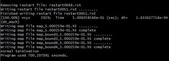
Final Temperature plot:
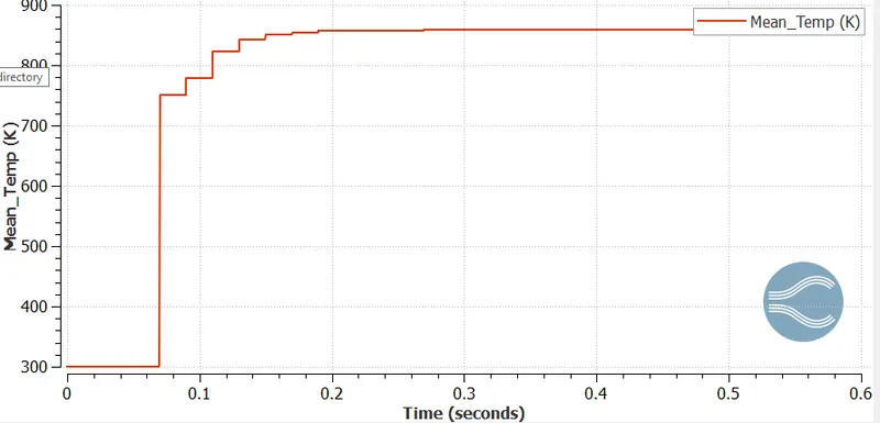
Final Temperature = 858.313K
Mesh 6
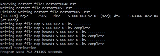
Completion Time:
Final Temperature plot:
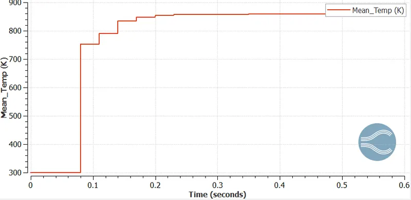
Final Temperature = 858.305K
It can be concluded that there is a direct impact of the supercycle stage interval on the smulation time and final temprature calculation.