Week 5 - Rayleigh Taylor Instability
The instability of a heavy fluid layer supported by a light one is generally known as Rayleigh-Taylor (RT) instability. It can occur under gravity and, equivalently, under an acceleration of the fluid systemin the direction toward the denser fluid.Water suspended atop oil is an everyday example of Rayleigh–Taylor instability, and it may be modeled by two completely plane-parallel layers of immiscible fluid, the more dense on top of the less dense one and both subject to the Earth's gravity.
Some practical CFD models that have been based on the mathematical analysis of Rayleigh Taylor waves are:
1. Richtmyer–Meshkov instability (RMI): The Richtmyer–Meshkov instability (RMI) occurs when two fluids of different density are impulsively accelerated. Normally this is by the passage of a shock wave. The development of the instability begins with small amplitude perturbations which initially grow linearly with time. This is followed by a nonlinear regime with bubbles appearing in the case of a light fluid penetrating a heavy fluid, and with spikes appearing in the case of a heavy fluid penetrating a light fluid. A chaotic regime eventually is reached and the two fluids mix. This instability can be considered the impulsive-acceleration limit of the Rayleigh–Taylor instability
2.Saffman–Taylor instability: The Saffman–Taylor instability, also known as viscous fingering, is the formation of patterns in a morphologically unstable interface between two fluids in a porous medium, described mathematically by Philip Saffman and G. I. Taylor in a paper of 1958. This situation is most often encountered during drainage processes through media such as soils. It occurs when a less viscous fluid is injected, displacing a more viscous fluid; in the inverse situation, with the more viscous displacing the other, the interface is stable and no instability is seen. Essentially the same effect occurs driven by gravity (without injection) if the interface is horizontal and separates two fluids of different densities, the heavier one being above the other: this is known as the Rayleigh-Taylor instability.
3.Kelvin–Helmholtz instability: The Kelvin–Helmholtz instability (after Lord Kelvin and Hermann von Helmholtz) typically occurs when there is velocity shear in a single continuous fluid, or additionally where there is a velocity difference across the interface between two fluids. A common example is seen when wind blows across a water surface; the instability constant manifests as waves. Kelvin-Helmholtz instabilities are also visible in the atmospheres of planets and moons, such as in cloud formations on Earth or the Red Spot on Jupiter, and the atmospheres (coronas) of stars, including the sun's.
4. Plateau–Rayleigh instability: The Plateau–Rayleigh instability, often just called the Rayleigh instability, explains why and how a falling stream of fluid breaks up into smaller packets with the same volume but less surface area. It is related to the Rayleigh–Taylor instability and is part of a greater branch of fluid dynamics concerned with fluid thread breakup. This fluid instability is exploited in the design of a particular type of ink jet technology whereby a jet of liquid is perturbed into a steady stream of droplets.
All the above stated instability types represents fluid as their medium and somehwere mixing is seen to be happening, and by Taking CFD approach to solve these problems would be easier to compare with the real life scenario so as to solve many real life problems.
The complete visualisation of this can be observed in Ansys by the follwing method. Also a new fluid isalso used in this case.
Initially in the space claim the 2 parts are made representing water and air and the model is shared inthe worspace tab.
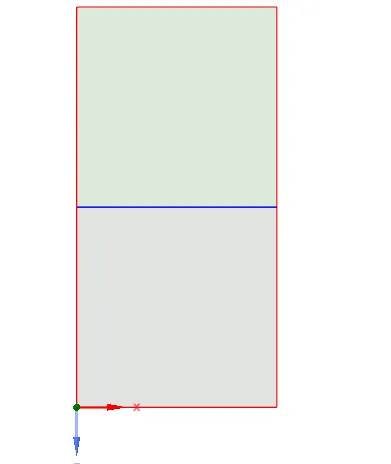
The meshing is done in the 3 cases which are discussed below.
The setup module is solved as follows:
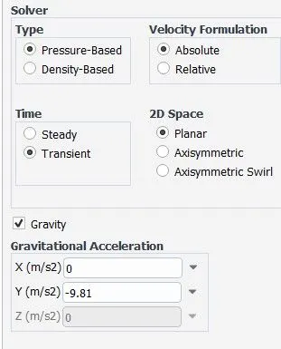
Transient solver along wih gravity enabled is taken into consideration
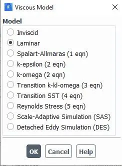
For the simplicity Laminar model was used
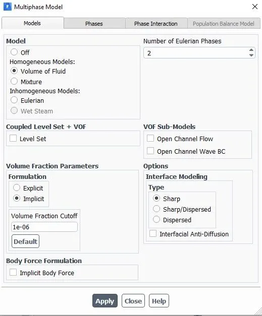
Volume of FLuid model with 2 phases is the main consideration
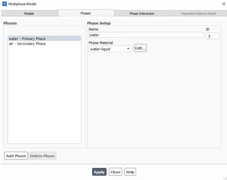
2 phases are given materials.
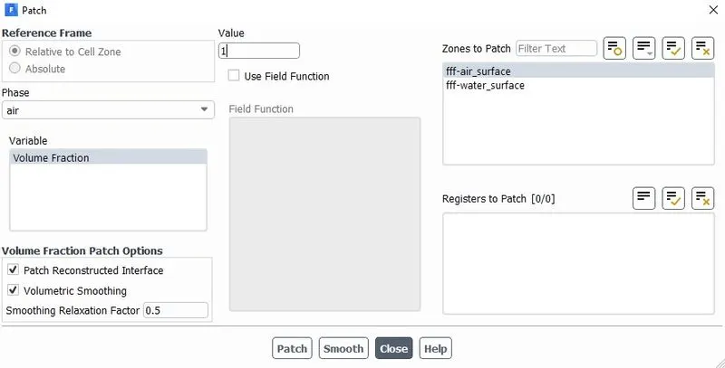
After initialisation the patch is defined for the 2 fluids.
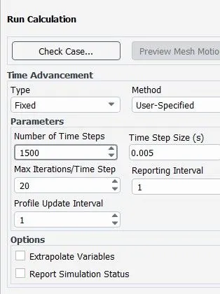
The simulation is run for 1500 time steps.
Case1: Baseline Mesh 0.5mm
https://drive.google.com/file/d/1ydIsvEX6rfPgHVEVQ089uj5RKpugk9Eh/view?usp=sharing
Case2: Mesh 0.2mm
https://drive.google.com/file/d/1fFFmDyEkSH0e3mfcfgJ7BgSJXyHmEqnu/view?usp=sharing
Case3: Mesh 0.25mm
https://drive.google.com/file/d/100BGN9Fwv2bjprgpngOL0PMB14g7m5MD/view?usp=sharing
Case4: simulation with water and user-defined material(density = 400 kg/m3, viscosity = 0.001 kg/m-s) for refined mesh.
https://drive.google.com/file/d/1Pu74O__4ns7ocwkI31dsm1H23_tJkVvz/view?usp=sharing
As from the above results it can be inferred that the more ideal like results can be obtained at finer mesh. So at finer mesh we can easily observe the bubles formation and the more accurate mixing behaviour of the 2 fluids.
A steady-state approach might not be suitable for these types of simulation, it turn out that the steady states are mostly unstable, which explains why they do not occur in the experiments. One should not be surprised. These stationary solutions, for larger amplitudes, do have an appearance suggestive of the bubbles and spikes . In steady state analysis we cant observe much result as we are getting in the transient state siulation because our aim is to get irregualrities and visualize them as if this is a real case.
The Atwood number (A) is a dimensionless number in fluid dynamics used in the study of hydrodynamic instabilities in density stratified flows. It is a dimensionless density ratio.
`A = (rho1-rho2)/(rho1+rho2)`
1. For air and water.
Air, Density = 1.225 kg/m^3
water, Density = 998.2 kg/m^3
A = 0.998
2. For water and new material
Water, density = 998.2 kg/m^3
New material, density = 400 kg/m^3
A = 0.428
Also from the above calculation it is clear that Atwood number with higher value close to 1 will make a larger bubble of the lighter fluid while the other atwood number value would mix more significantly. It is also seen from the above results videos too.