Week 6 - Multivariate Newton Rhapson Solver

Solving the non-linear coupled equations.

The equations are given as:

`(dy1)/dt= -0.04*y1 + 10^4*y2*y3`

`(dy2)/dt = 0.04*y1 - 10^4*y2*y3 - 3*10^7*y2^2`

`(dy3)/dt = 3*10^7*y2^2`

To solve the above set of equations jacobian and implicit Euler solver are used.

Implicit Euler: For solving the equations backward differencing scheme is used. The backward differencing can be written as:

`dy/dt=f(x,y)`

`(y^n - y^(n-1))/dt=f(x,y)`

After applying the backward scheme given equations become,

`y1_(old)-y1+dt*(-0.04*y1 + 10^4 * y2 * y3)=0`

`y2_(old) - y2 + dt*(0.04*y1- 10^4*y2*y3 - 3*10^7*y2^2)=0`

`y3_(old) - y3 + dt*(3*10^7*y2^2)=0`

The above equations will be solved by using the jacobian matrix method.

`Y_(updated)=Y_(old)-alpha*(J^(-1)*F)^n`

where, `F=[[f1],[f2],[f3]]`

`J=[[(df1)/(dy1),(df1)/(dy2),(df1)/(dy3)],[(df2)/(dy1),(df2)/(dy2),(df2)/(dy3)],[(df3)/(dy1),(df3)/(dy2),(df3)/(dy3)]]`

The code to solve the above problem is shown below for the complete time of 10 minutes is shown below.

The initial values are: y1 = 1, y2 = 0, y3 = 0

"""
Program to solve 3 non linear coupled problems

dy1/dt= -0.04*y1 + 10^4*y2*y
dy2/dt = 0.04*y1 - 10^4*y2*y3 - 3*10^7*y2^2
dy3/dt = 3*10^7*y2^2

Modules required:
1. Numpy: Matrix multiplicaton
2. Inverse of Matrix
"""
import numpy as np
from numpy.linalg import inv
import matplotlib.pyplot as plt

def f1(y1, y2, y3, y1_old,dt):

	return y1_old-y1+dt*(-0.04*y1 + pow(10,4) * y2 * y3)

def f2(y1, y2, y3, y2_old,dt):

	return y2_old - y2 + dt*(0.04*y1- pow(10,4)*y2*y3 - 3*pow(10,7)*pow(y2,2))

def f3(y1, y2, y3, y3_old,dt):

	return y3_old - y3 + dt*(3*pow(10,7)*pow(y2,2))



def jacobian(y1, y2, y3, y1_old, y2_old, y3_old, dt, h):

	h= 1e-6;

	J = np.ones((3,3))

	J[0,0] = (f1(y1+h,y2,y3,y1_old,dt)-f1(y1,y2,y3,y1_old,dt))/h;
	J[0,1] = (f1(y1,y2+h,y3,y1_old,dt)-f1(y1,y2,y3,y1_old,dt))/h;
	J[0,2] = (f1(y1,y2,y3+h,y1_old,dt)-f1(y1,y2,y3,y1_old,dt))/h;

	#J[1,0]= (f2(y1+h,y2,y3,y1_old,dt)-f2(y1,y2,y3,y2_old,dt))/h;
	J[1,0]= (f2(y1+h,y2,y3,y2_old,dt)-f2(y1,y2,y3,y2_old,dt))/h;
	#J[1,1]= (f2(y1,y2+h,y3,y1_old,dt)-f2(y1,y2,y3,y2_old,dt))/h;
	J[1,1]= (f2(y1,y2+h,y3,y2_old,dt)-f2(y1,y2,y3,y2_old,dt))/h;
	#J[1,2]= (f2(y1,y2,y3+h,y1_old,dt)-f2(y1,y2,y3,y2_old,dt))/h;
	J[1,2]= (f2(y1,y2,y3+h,y2_old,dt)-f2(y1,y2,y3,y2_old,dt))/h;

	# Same definition missing theere
	J[2,0]= (f3(y1+h,y2,y3,y3_old,dt)-f3(y1,y2,y3,y3_old,dt))/h;
	J[2,1]= (f3(y1,y2+h,y3,y3_old,dt)-f3(y1,y2,y3,y3_old,dt))/h;
	J[2,2]= (f3(y1,y2,y3+h,y3_old,dt)-f3(y1,y2,y3,y3_old,dt))/h;

	return J

#Defining initial guess
y1_old=1;
y2_old=0;
y3_old=0;

#including error
error = 9e9

#column vector
y_old = np.ones((3,1))
y_old[0]=y1_old
y_old[1]=y2_old
y_old[2]=y3_old

#Making a copy

F= np.copy(y_old)

alpha = 1
tol = 1e-6
h= 1e-6;
dt = 1;
t=600;
n=int(t/dt);
itt = []
error_up = []
y1_new=[]
y2_new=[]
y3_new=[]
#Newton Raphson starting 
iter =1
total_iter=1
for  i in range(0,n):
	while error>tol:
		#for computing jacobian old values are used
		J  =jacobian(y_old[0], y_old[1], y_old[2], y1_old, y2_old, y3_old, dt,h)

		F[0]= f1(y_old[0], y_old[1], y_old[2],y1_old,dt);
		F[1]= f2(y_old[0], y_old[1], y_old[2],y2_old,dt);
		F[2]= f3(y_old[0], y_old[1], y_old[2],y3_old,dt);

		#computing new values
		y_new = y_old -alpha*np.matmul(inv(J), F)

		#max abs error
		error = np.max(np.abs(y_new-y_old))
		print(error)
		#updating
		y_old = y_new

		
		#log message
	log_message = 'iteration  = {0} y1 = {1} y2 = {2} y3 = {3}'.format(iter, y1_old, y2_old, y3_old)

	print(log_message)
		
	iter = iter+1

	error_up.append(error)

	

	y_old=y_new
	y1_old=y_new[0]
	y2_old=y_new[1]
	y3_old=y_new[2]

		#final results
	y1_new.append(y_new[0])
	y2_new.append(y_new[1])
	y3_new.append(y_new[2])
	itt.append(iter)
	error = 9e9

plt.plot(y1_new)
plt.plot(y2_new)
plt.plot(y3_new)
plt.show()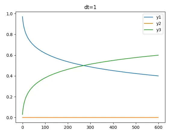

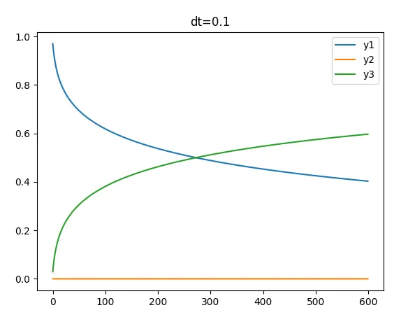
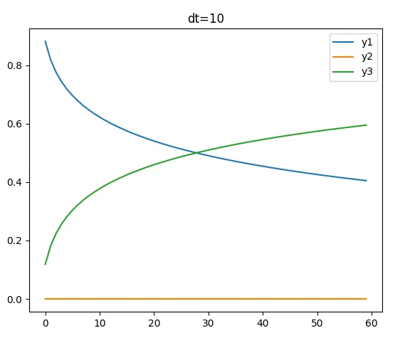
Three different time steps are used in solving the problem which are 0.1, 1 & 10 and the number of iterations in each of the cases are 6000, 600, 60. So to get a converged result near the analytical one some amount of calculations needs to be done and thus 0.1 time step can be tested as the ideal,