Week 3 - Taylor table method and Matlab code
Deriving fourth order approximations for second order derivative:
1. Central differencing : In central differencing scheme, we take in consideration two grid points on the left side and two gid points on right side. we can rewrite our second-derivative as
`delta^2 x//delta x^2 = a *f(i-2) + b* f(i-1) + c*f(i) + d*f(i+1) + e*f(i+2)`
On further expanding the above terms in form of taylor series expansion we get an output table as
| f(i) | `Deltax*f'(i)` | `Deltax^2 * f''(i)` | `Deltax^3 * f'''(i)` | `Deltax^4 * f^(IV)(i)` | `Deltax^5*f^V(i)` | `Deltax^6*f^(VI)(i)` | |
| a*f(i-2) | a | -2a | 2a | -8a/6 | 16a/24 | -32a/120 | 64a/240 |
| b*f(i-1) | b | -b | b/2 | -b/6 | b/24 | -b/120 | b/240 |
| c*f(i) | c | 0 | 0 | 0 | 0 | 0 | 0 |
| d*f(i+1) | d | d | d/2 | d/6 | d/24 | d/120 | d/240 |
| e*f(i+2) | e | 2e | 2e | 8e/6 | 16e/24 | 32e/120 | 64e/240 |
On Equating the these linear equations with LHS i.e our second order differential, we get
a+b+c+d+e=0
-2a - b + d + 2e = 0
2a + b/2 + d/2 + 2e = 1
-8a/6 - b/ + d/6 + 8e/6 = 0
16a/24 + b/24 + d/24 + 16e/24 = 0
Solving these equations as linear eqaution solver on Matlab,
we solve it as
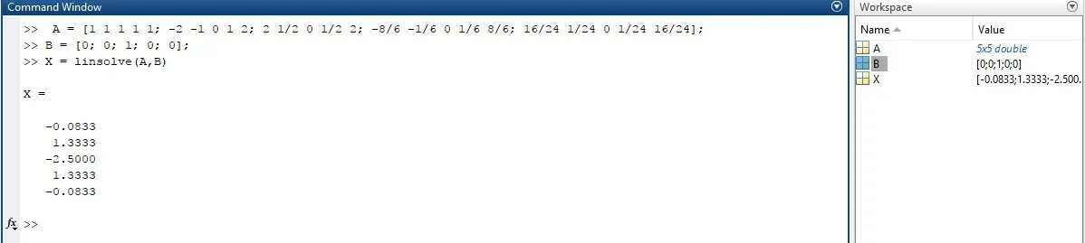
We get the values as
a = -0.0833
b = 1.3333
c = -2.5
d = 1.333
e = -0.08333
Now rewriting these in our main equation ,
`delta^2 x//delta x^2 = a *f(i-2) + b* f(i-1) + c*f(i) + d*f(i+1) + e*f(i+2)` = expansion of each term as fourier series`
After substitution we get,
`delta^2 x//delta x^2 = (a *f(i-2) + b* f(i-1) + c*f(i) + d*f(i+1) + e*f(i+2))//(Deltax)^2 = (...)f''(x) + O(Deltax)^4`
SO we get our result as fourth order truncation error.
2. Skewed Right approximation:
In Skewed Right approximation, we take in consideration 5 grid points on the right side as we considered
No. of grid points on skewed = order of approximation reqd. + order of differentiation
. we can rewrite our second-derivative as
`delta^2 x//delta x^2 = a *f(i) + b* f(i+1) + c*f(i+2) + d*f(i+3) + e*f(i+4) + f*f(i+5)`
On further expanding the above terms in form of taylor series expansion we get an output table as
| f(i) | `Deltax*f'(i)` | `Deltax^2 * f''(i)` | `Deltax^3 * f'''(i)` | `Deltax^4 * f^(IV)(i)` | `Deltax^5*f^V(i)` | |
| a*f(i) | a | 0 | 0 | 0 | 0 | 0 |
| b*f(i+1) | b | b | b/2 | b/6 | b/24 | b/120 |
| c*f(i+2) | c | 2c | 4c/2 | 8c/6 | 16c/24 | 32c/120 |
| d*f(i+3) | d | 3d | 9d/2 | 27d/6 | 81d/24 | 243d/120 |
| e*f(i+4) | e | 4e | 16e/2 | 64e/6 | 256e/24 | 1024e/120 |
| f*f(i+5) | f | 5f | 25f/2 | 125f/6 | 625e/24 | 3125f/120 |
On Equating the these linear equations with LHS i.e our second order differential, we get
a +b+ c+ d+ e+ f =0
b + 2c + 3d+ 4e + 5f = 0
b/2 + 4c/2 + 9d/2 + 16e/2 + 25f/2 = 1
b/6 + 8c/6 + 27d/6 + 64e/6 + 125f/6 = 0
b/24 + 16c/24 + 81d/24 + 256e/24 + 625f/24 = 0
b/120 + 32c/120 + 243d/120 + 1024e/120 + 3125f/120 = 0
Solving these equations as linear eqaution solver on Matlab,
we solve it as
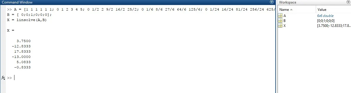
a = 3.7500
b = -12.8333
c = 17.8333
d = -13
e= 5.08333
f = -0.8333
Now rewriting these in our main equation ,
`delta^2 x//delta x^2 = a *f(i) + b* f(i+1) + c*f(i+2) + d*f(i+3) + e*f(i+4) + f*f(i+5)` = = expansion of each term as fourier series
After substitution we get,
`delta^2 x//delta x^2 = a *f(i) + b* f(i+1) + c*f(i+2) + d*f(i+3) + e*f(i+4) + f*f(i+5)`= (...)f''(x) + O(Deltax)^4`
SO we get our result as fourth order truncation error.
3. Skewed Left approximation:
In Skewed Left approximation, we take in consideration 5 grid points on the left side as we considered
No. of grid points on skewed = order of approximation reqd. + order of differentiation
. we can rewrite our second-derivative as
`delta^2 x//delta x^2 = a *f(i) + b* f(i-1) + c*f(i-2) + d*f(i-3) + e*f(i-4) + f*f(i-5)`
On further expanding the above terms in form of taylor series expansion we get an output table as
| f(i) | `Deltax*f'(i)` | `Deltax^2 * f''(i)` | `Deltax^3 * f'''(i)` | `Deltax^4 * f^(IV)(i)` | `Deltax^5*f^V(i)` | |
| a*f(i) | a | 0 | 0 | 0 | 0 | 0 |
| b*f(i+1) | b | -b | b/2 | -b/6 | b/24 | -b/120 |
| c*f(i+2) | c | -2c | 4c/2 | -8c/6 | 16c/24 | -32c/120 |
| d*f(i+3) | d | -3d | 9d/2 | -27d/6 | 81d/24 | -243d/120 |
| e*f(i+4) | e | -4e | 16e/2 | -64e/6 | 256e/24 | -1024e/120 |
| f*f(i+5) | f | -5f | 25f/2 | -125f/6 | 625e/24 | -3125f/120 |
On Equating the these linear equations with LHS i.e our second order differential, we get
a +b+ c+ d+ e+ f =0
-b - 2c - 3d- 4e - 5f = 0
b/2 + 4c/2 + 9d/2 + 16e/2 + 25f/2 = 1
-b/6 - 8c/6 - 27d/6 - 64e/6 - 125f/6 = 0
b/24 + 16c/24 + 81d/24 + 256e/24 + 625f/24 = 0
-b/120 - 32c/120 - 243d/120 - 1024e/120 - 3125f/120 = 0
we solve it as
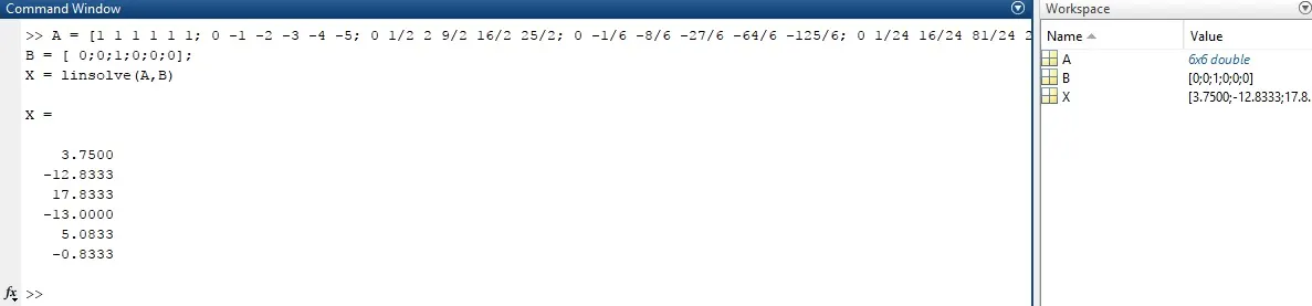
a = 3.7500
b = -12.8333
c = 17.8333
d = -13.0000
e = 5.0833
f = -0.8333
Now writing the function in matlab as
1. For central differencing
function out = ass_fourth_order_approx_function_second_derivative_central_diff(x,dx)

% analytical derivative = exp(x)*cos(x)
% f'(x) = exp(x)*cos(x) - exp(x)*sin(x)
% f''(x) = -2*exp(x) * sin(x)

analytical_derivative = -2*exp(x) * sin(x);

% numerical derivative
differencing = (-0.0833*(exp(x-(2*dx)))*(cos(x-(2*dx)))) + (1.333)*(exp(x-dx))*(cos(x-dx)) -(2.5)*(exp(x))*(cos(x)) +(1.333)*(exp(x+dx))*(cos(x+dx)) -(0.08333)*(exp(x+(2*dx)))*(cos(x+(2*dx)));

out = abs(differencing - analytical_derivative);

end
2. For Left skewed
function out = ass_fourth_order_approx_function_second_derivative_skewed_left(x,dx)

% analytical derivative = exp(x)*cos(x)
% f'(x) = exp(x)*cos(x) - exp(x)*sin(x)
% f''(x) = -2*exp(x) * sin(x)

analytical_derivative = -2*exp(x) * sin(x);

% numerical derivative
differencing = (0.091046)*(exp(x))*(cos(x)) -(0.33088)*exp((x+dx))*cos((x+dx))+ (0.058691)*(exp(x+(2*dx)))*(cos(x+(2*dx))) +(2.250941)*(exp(x+(3*dx)))*(cos(x+(3*dx)))-(3.457487)*(exp(x+(4*dx)))*(cos(x+(4*dx))) +(1.505079)*(exp(x+(5*dx)))*(cos(x+(5*dx)));

out = abs(differencing - analytical_derivative);

end
3. For right skewed
function out = ass_fourth_order_approx_function_second_derivative_skewed_right(x,dx)

% analytical derivative = exp(x)*cos(x)
% f'(x) = exp(x)*cos(x) - exp(x)*sin(x)
% f''(x) = -2*exp(x) * sin(x)

analytical_derivative = -2*exp(x) * sin(x);

% numerical derivative
differencing = (3.7500)*(exp(x))*(cos(x)) -(12.8333)*(exp(x+dx))*(cos(x+dx)) +17.8333*exp(x+(2*dx))*cos(x+(2*dx)) -13*exp(x+(3*dx))*cos(x+(3*dx)) +5.08333*exp(x+(4*dx))*cos(x+(4*dx)) -0.8333*exp(x+(5*dx))*cos(x+(5*dx));

out = abs(differencing - analytical_derivative);

end
4. Our main function
close all
clc
%given values
x = pi/3;
dx = linspace(pi/10, pi/30, 2000);

for i= 1:length(dx)

    central_diff(i) = ass_fourth_order_approx_function_second_derivative_central_diff(x,dx(i));
    left_skew(i) = ass_fourth_order_approx_function_second_derivative_skewed_left(x,dx(i));
    right_skew(i) = ass_fourth_order_approx_function_second_derivative_skewed_right(x,dx(i));
end


%Plotting
loglog(dx,central_diff)
hold on
loglog(dx,left_skew,'r')
hold on
plot(dx,right_skew,'g')
xlabel('dx')
ylabel('error')
legend('central diff','left skew','right skew')
In the result we get a plot which is,
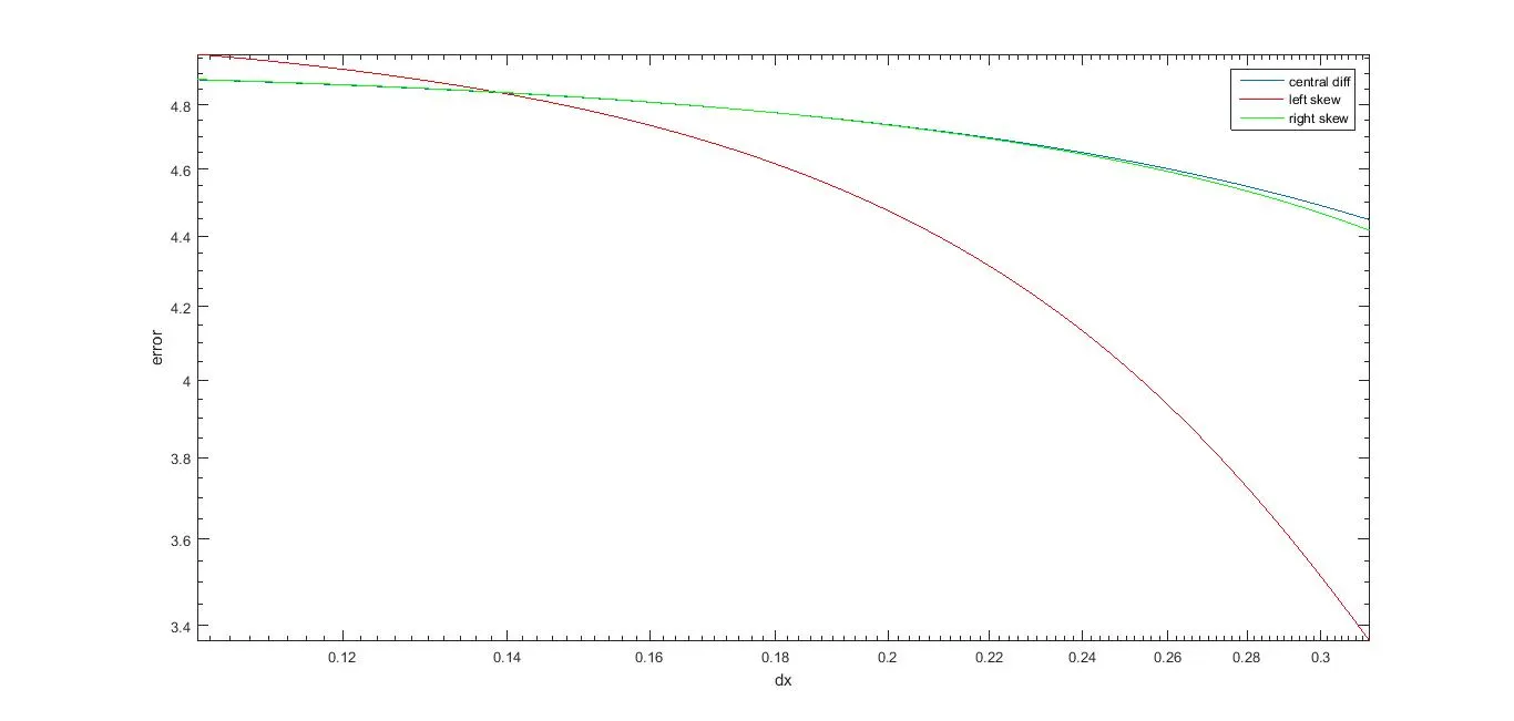
From the above plot it is clear that skewed plot will always have lesser error and would be close enought to real result. Also it can be inferred that it will always be benfiial for one to adopt a skewed scheme inspite of selecting a central differncing scheme.