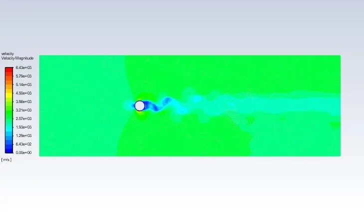
Week 2 - Flow over a Cylinder.

The flow past a circular cylinder is associated with various instabilities. These instabilities involve the wake, separated shear layer and boundary layer. Williamson1 has given a comprehensive description of the flow phenomena at different Reynolds numbers (Re). Upto Re ∼ 47, the flow is steady with two symmetric vortices on each side of the wake center line. The first wake instability, manifestation of a Hopf bifurcation, occurs at Re ∼ 47. For Re > 47, although it remains laminar, the flow becomes unsteady and asymmetric. Von Karman vortex shedding is observed for slightly larger Re. At Re ∼ 190, three-dimensional instabilities, such as formation of vortex loops, deformation of primary vortices and stream wise and span wise vortices, appear in wake. The wake flow undergoes a series of complex three-dimensional instabilities, eventually making it turbulent. Beyond a certain critical Re, the shear layer separating from the upper and lower surface of the cylinder, starts becoming unstable via the Kelvin-Helmholtz mode of instability. The transition point, beyond which the separated layer becomes unstable, moves upstream with increase in Re. At Re ∼ 2 × 105
, the boundary layer on the cylinder surface undergoes a transition from laminar to turbulent. This transition leads to a delay of the separation of flow from the cylinder surface causing a substantial reduction in the drag force that the cylinder experiences. This is often referred to as Drag crisis.

Setting up the flow over cylinder case:

Initially the 2d grid is made and the pull command is used to make our geometry complete.

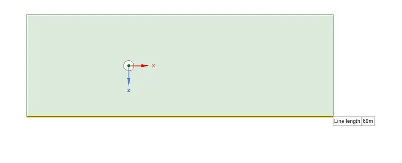The mesh is now defined on the geometry with other parameters as-

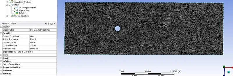
In the meshing part the mesh size is kept 0.25m. Also triangular mesh is adopted. Inflation of 6 layers is done around the circle.

Setting up the case:

The various inputs taken are as-

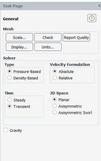
Selecting the solver(as here transient is selected)

Selecting the material i.e at our inlet .

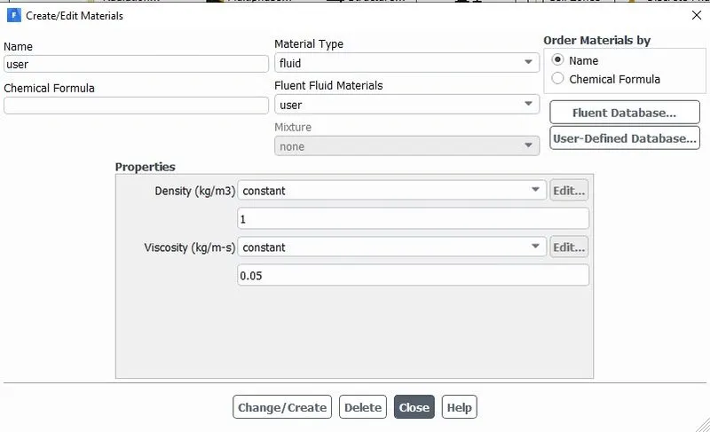
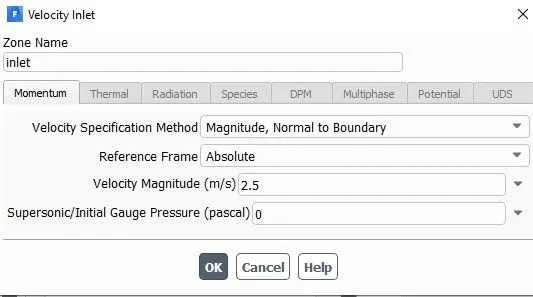
Selecting the inlet and outlet values

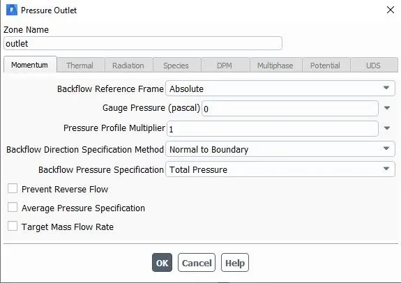
The parameters taken at outlet are-

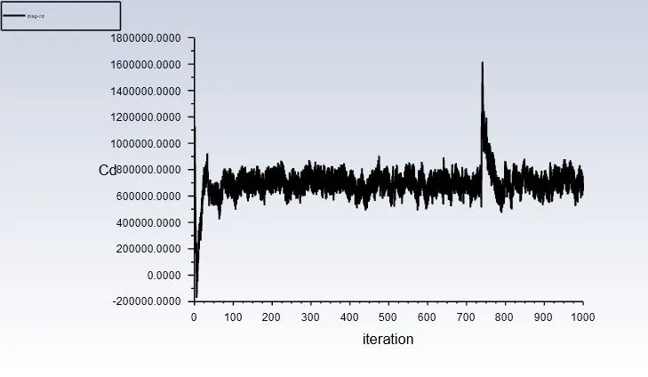
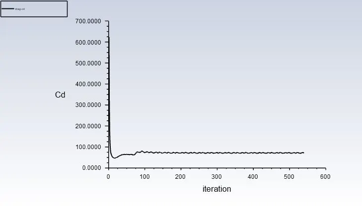
1. The drag coefficient is a number that aerodynamicists use to model all of the complex dependencies of shape, inclination, and flow conditions on aircraft drag. This equation is simply a rearrangement of the drag equation where we solve for the drag coefficient in terms of the other variables. The drag coefficient Cd is equal to the drag D divided by the quantity: density r times half the velocity V squared times the reference area A.

Cd = D / (A * .5 * r * V^2)

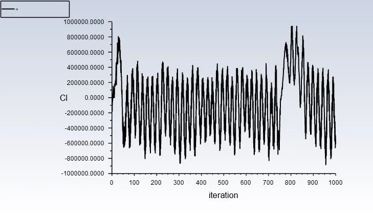
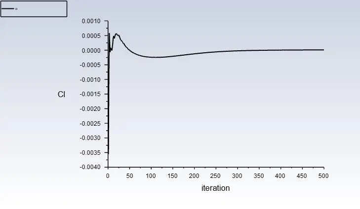
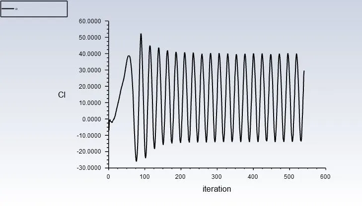
2. The lift coefficient is a number that aerodynamicists use to model all of the complex dependencies of shape, inclination, and some flow conditions on lift. This equation is simply a rearrangement of the lift equation where we solve for the lift coefficient in terms of the other variables. The lift coefficient Cl is equal to the lift L divided by the quantity: density r times half the velocity V squared times the wing area A.

Cl = L / (A * .5 * r * V^2)

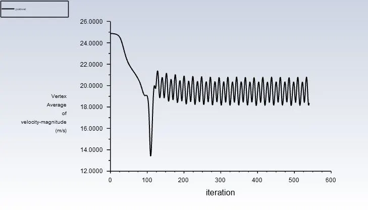
3. In dimensional analysis, the Strouhal number (St, or sometimes Sr to avoid the conflict with the Stanton number) is a dimensionless number describing oscillating flow mechanisms. The parameter is named after Vincenc Strouhal, a Czech physicist who experimented in 1878 with wires experiencing vortex shedding and singing in the wind.The Strouhal number is an integral part of the fundamentals of fluid mechanics.

The Strouhal number is often given as

PART-I

1. Simulate the flow with the steady and unsteady case and calculate the Strouhal Number for Re= 100.

For Steady state solver:

Material : Density-1kg/m^3

Viscosity-0.05kg/m-s

Inlet Velocity: 2.5 m/s

Outlet Pressure: 0 Pa(gauge)

Solver: Steady

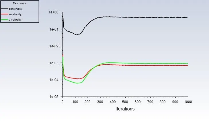
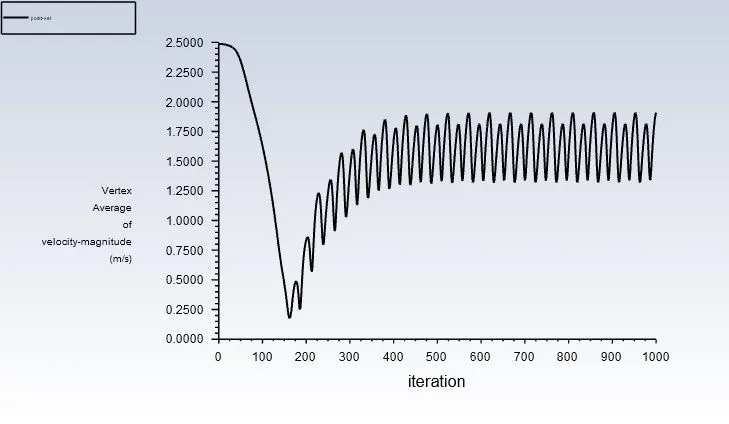
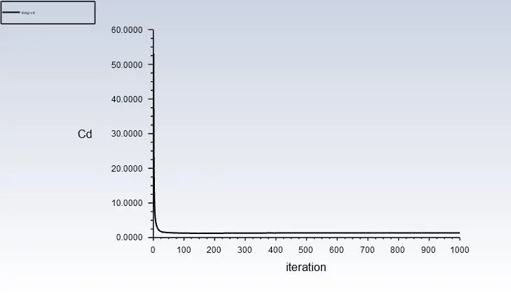
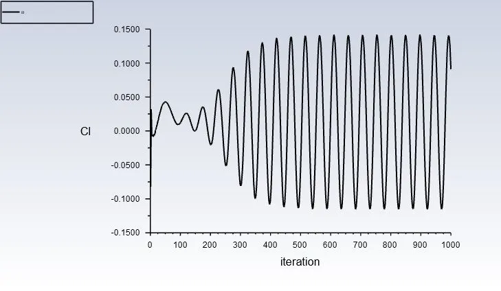
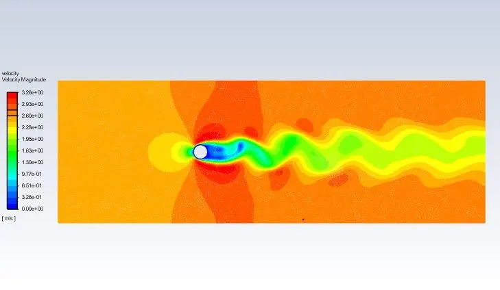
For UnSteady state solver:

Material : Density-1kg/m^3

Viscosity-0.05kg/m-s

Inlet Velocity: 2.5 m/s

Outlet Pressure: 0 Pa(gauge)

Solver: Transient

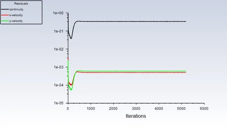
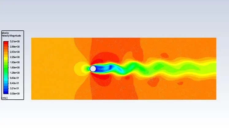
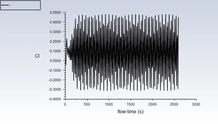
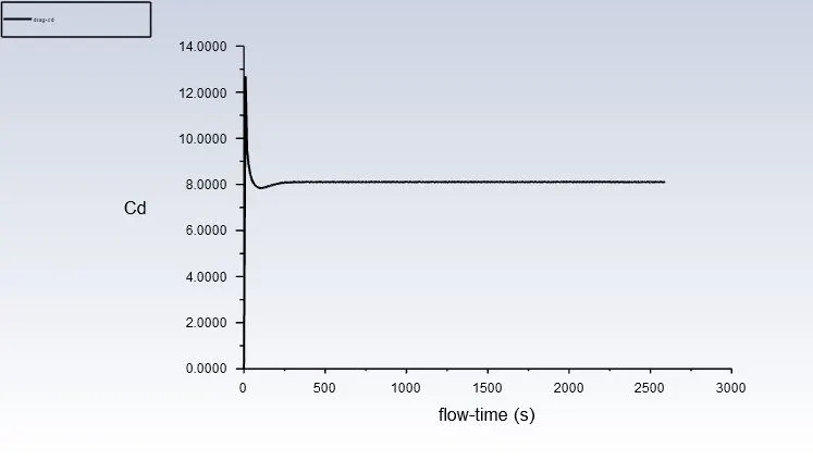
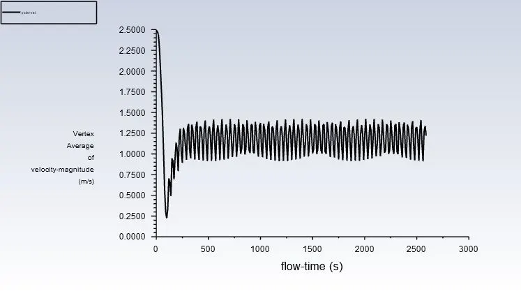
From above Te strouhal no. is calculated as : 0.1786

PART-II

1. Calculate the coefficient of drag and lift over a cylinder by setting the Reynolds number to 10,100,1000,10000 & 100000. (Run with steady solver)
2. Discuss the effect of Reynolds number on the coefficient of drag. [ Results should be validated with any standard literature and error should be within 5 %]

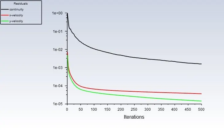
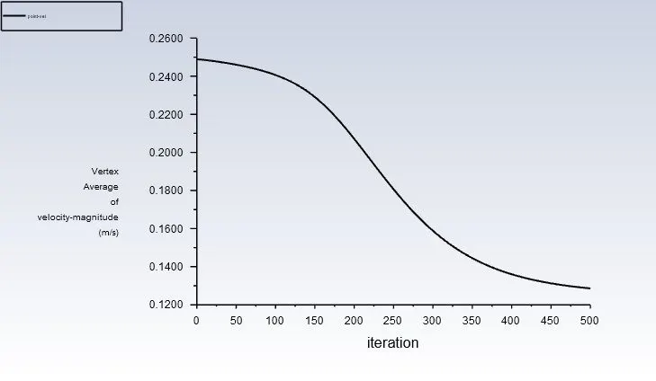
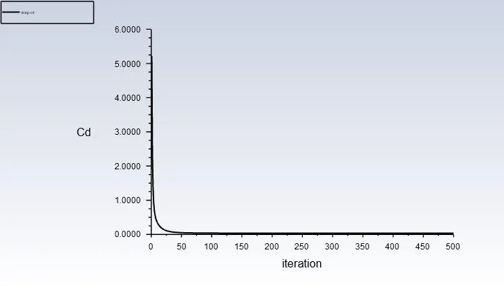
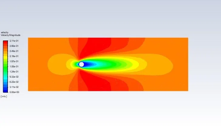
RE10

Material : Density-1kg/m^3

Viscosity-0.05kg/m-s

Inlet Velocity: 0.25 m/s

Outlet Pressure: 0 Pa(gauge)

Solver: Steady

RE100

Material : Density-1kg/m^3

Viscosity-0.05kg/m-s

Inlet Velocity: 2.5 m/s

Outlet Pressure: 0 Pa(gauge)

Solver: Steady

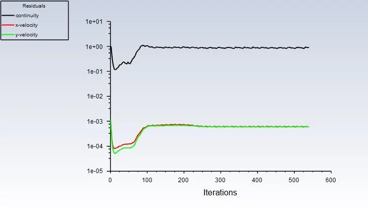
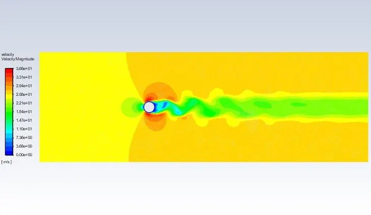
RE1000

Material : Density-1kg/m^3

Viscosity-0.05kg/m-s

Inlet Velocity: 25 m/s

Outlet Pressure: 0 Pa(gauge)

Solver: Steady

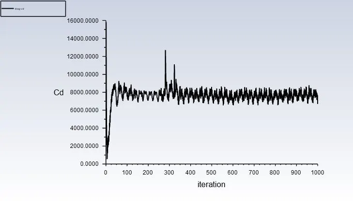
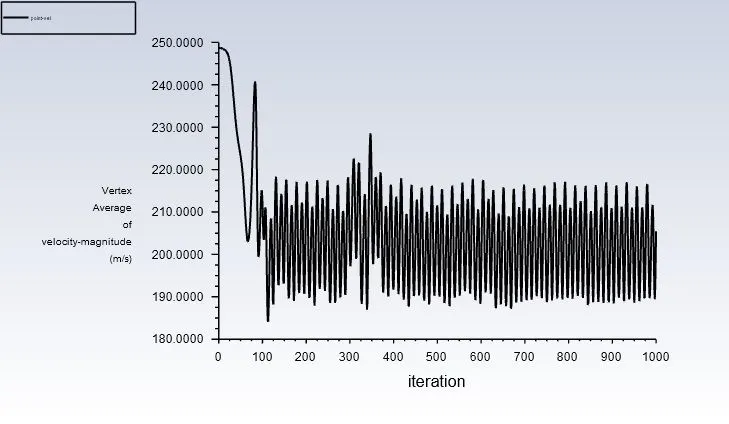
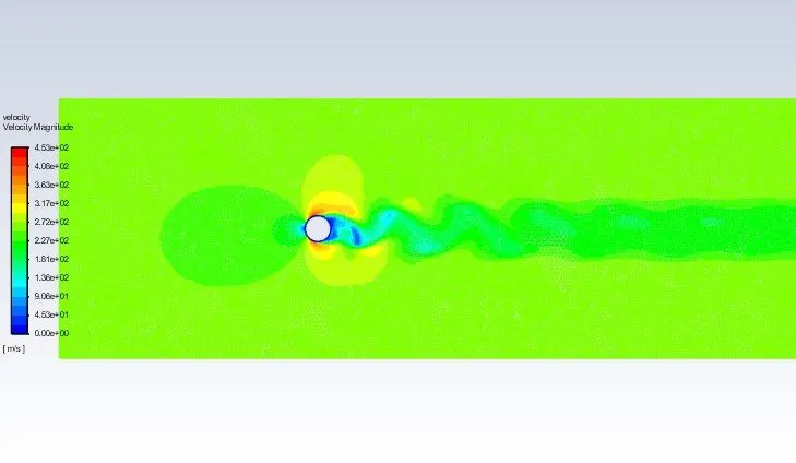
RE10000

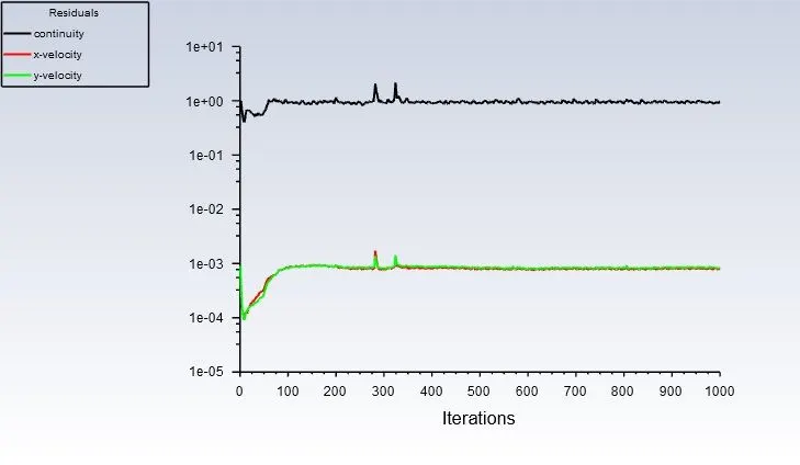
Material : Density-1kg/m^3

Viscosity-0.05kg/m-s

Inlet Velocity: 250 m/s

Outlet Pressure: 0 Pa(gauge)

Solver: Steady

RE100000

Material : Density-1kg/m^3

Viscosity-0.05kg/m-s

Inlet Velocity: 2500 m/s

Outlet Pressure: 0 Pa(gauge)

Solver: Steady