Week 5.1 - Mid term project - Solving the steady and unsteady 2D heat conduction problem
AIM
To understand the steady and unsteady heat conduction over a domain by considering iterative solvers like Jacobian, Gauss-Seidel and Successive_Over_Relaxation and to write a MATLAB program to do the same.
THEORY & BOUNDARY CONDITIONS
The general,transient 2D equation of conduction is `(delT)/(delt)=alpha((del^2T)/(delx^2)+(del^2T)/(dely^2))`
where,T->temperature
For a steady case,the above equation becomes `(del^2T)/(delx^2)+(del^2T)/(dely^2) =0`
For an unsteady case, we have to use implicit and explicit schemes whereas, for a steady one, we need not worry.
The program is written individually for each solver, first for a steady case and then for an unsteady case and the graphs are plotted.
By solving the above equation and discretizing, let us assume (i,j) as the point P. Then consequently,
| i,j+1 T | ||
| i-1,j L | i,j P | i+1,j R |
| i,j-1 B |
(i-1,j)=L (i,j+1)=T
(i+1,j)=R (i,j-1)=B
`(underset(L)(T) - 2*underset(P)(T)+underset(R)(T))/(Deltax)^2 + (underset(T)(T) - 2*underset(P)(T)+underset(B)(T))/(Deltay)^2 =0`
Simplifying the above expression,we get
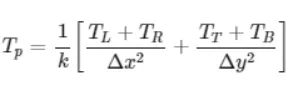
where,
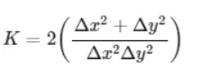
To solve this equation on a domain, consider a square domain with dx=dy=10 units(say), and divide this zone into 10 equal intervals. The next step involves applying boundary conditions which are
Temperature on the left wall=400K
Temperature on the top wall=600K
Temperature on the right wall=800K
Temperature on the bottom wall=900K
Temperature at the corners can be determined as the average of the two values.
To check whether the solution converges, use a while loop specifying a tolerance value.
STEADY CASE
JACOBI ITERATION:
In this method, the old values are used throughout one entire iteration. Once one iteration is completed, the new values are updated and are used in the next iterations and so forth i.e to calculate at `underset(i+1,j)(T)` we only use the old values.
%To solve steady state conduction equation d^2T/dx^2 +d^2T/dy^2 =0

%Initial values
n_x=10;                %no of nodes in x direction
n_y=10;                %no of nodes in y direction
x=linspace(1,n_x,10);  %x axis
y=linspace(1,n_y,10);  %y axis
dx=x(2)-x(1);          %to calculate dx
dy=y(2)-y(1);          %to calculate dy
k=2*((dx^2 +dy^2)/((dx*dy)^2));
%Boundary conditions
T=350*ones(n_x,n_y);      %Initial Temperature
T(1,2:n_x-1)=600;         %Temperature at the top is 600K
T(10,2:n_x-1)=900;        %Temperature at the bottom is 900K
T(2:n_y-1,1)=400;         %Temperature on the left side is 400K
T(2:n_y-1,10)=800;        %Temperature on the right side is 800K

%Temperatures at corners
T(1,1)=500;
T(1,10)=700;
T(10,1)=650;
T(10,10)=850;
T_old=T;
T_initial=T;
tolerance=1e-4;   %So as to make sure that the error is below this value
error=10e5;
w=1.2;
%Convergence Loop
iter=0;       %to calculate number of iterations
while error>tolerance
    for i=2:n_x-1       %Because Boundary conditions are known at 1 and 10
        for j=2:n_y-1
            T(i,j)=((T_old(i-1,j)+T_old(i+1,j))/(k*(dx^2))) + ((T_old(i,j-1)+T_old(i,j+1))/(k*(dy^2))) ;
        end
    end
    iter=iter+1;
    error=max(max(abs(T_old-T)));
    T_old=T;
    figure(1)
    contourf(x,y,T)
    clabel(contourf(x,y,T))
    colorbar
    colormap(jet)
    set(gca,'ydir','reverse')
    xlabel('X-axis');
    ylabel('Y-axis');
    title(sprintf('Number of jacobi iterations:%d',iter));
    pause(0.03)
end
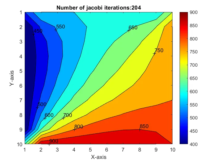
PLOT
GAUSS SEIDEL ITERATION:
The difference between the gauss seidel and Jacobi methods is that the values get updated within the loop. This methods usually results in quicker solutions.
%To solve steady state conduction equation d^2T/dx^2 +d^2T/dy^2 =0

%Initial values
n_x=10;                %no of nodes in x direction
n_y=10;                %no of nodes in y direction
x=linspace(1,n_x,10);  %x axis
y=linspace(1,n_y,10);  %y axis
dx=x(2)-x(1);          %to calculate dx
dy=y(2)-y(1);          %to calculate dy
k=2*((dx^2 +dy^2)/((dx*dy)^2));
%Boundary conditions
T=350*ones(n_x,n_y);      %Initial Temperature
T(1,2:n_x-1)=600;         %Temperature at the top is 600K
T(10,2:n_x-1)=900;        %Temperature at the bottom is 900K
T(2:n_y-1,1)=400;         %Temperature on the left side is 400K
T(2:n_y-1,10)=800;        %Temperature on the right side is 800K

%Temperatures at corners
T(1,1)=500;
T(1,10)=700;
T(10,1)=650;
T(10,10)=850;
T_old=T;
T_initial=T;
tolerance=1e-4;   %So as to make sure that the error is below this value
error=10e5;
w=1.2;
%Convergence Loop
iter=0;       %to calculate number of iterations
while error>tolerance
    for i=2:n_x-1       %Because Boundary conditions are known at 1 and 10
        for j=2:n_y-1
            T(i,j)=((T(i-1,j)+T_old(i+1,j))/(k*(dx^2))) + ((T(i,j-1)+T_old(i,j+1))/(k*(dy^2))) ;
        end
    end
    iter=iter+1;
    error=max(max(abs(T_old-T)));
    T_old=T;
    figure(1)
    contourf(x,y,T)
    clabel(contourf(x,y,T))
    colorbar
    colormap(jet)
    set(gca,'ydir','reverse')
    xlabel('X-axis');
    ylabel('Y-axis');
    title(sprintf('Number of Gauss-Seidel iterations:%d',iter));
    pause(0.03)
end
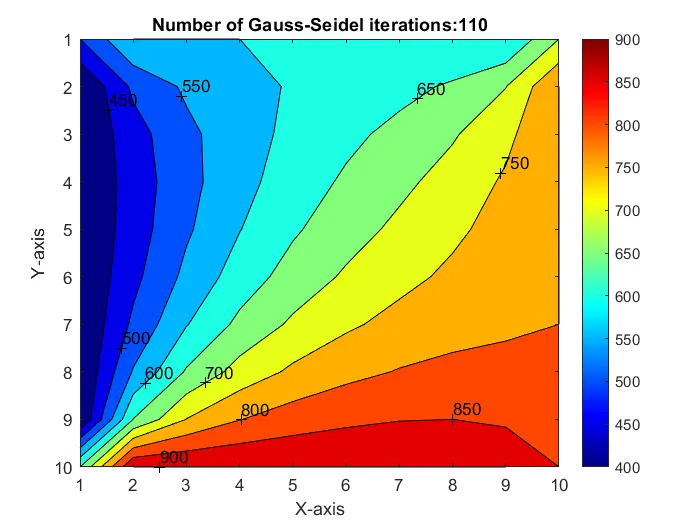
PLOT
SUCCESSIVE OVER-RELAXATION:
In the Successive overrelaxation method, we define a variable `omega` which is the relaxation factor.
When `omega`>1, it is called as overrelaxation method.
When `omega`<1, it is called under relaxation method.
We choose an appropriate value for `omega` such that the solution converges.
%To solve steady state conduction equation d^2T/dx^2 +d^2T/dy^2 =0

%Initial values
n_x=10;                %no of nodes in x direction
n_y=10;                %no of nodes in y direction
x=linspace(1,n_x,10);  %x axis
y=linspace(1,n_y,10);  %y axis
dx=x(2)-x(1);          %to calculate dx
dy=y(2)-y(1);          %to calculate dy
k=2*((dx^2 +dy^2)/((dx*dy)^2));
%Boundary conditions
T=350*ones(n_x,n_y);      %Initial Temperature
T(1,2:n_x-1)=600;         %Temperature at the top is 600K
T(10,2:n_x-1)=900;        %Temperature at the bottom is 900K
T(2:n_y-1,1)=400;         %Temperature on the left side is 400K
T(2:n_y-1,10)=800;        %Temperature on the right side is 800K

%Temperatures at corners
T(1,1)=500;
T(1,10)=700;
T(10,1)=650;
T(10,10)=850;
T_old=T;
T_initial=T;
tolerance=1e-4;   %So as to make sure that the error is below this value
error=10e5;
w=1.2;
%Convergence Loop
iter=0;       %to calculate number of iterations
while error>tolerance
    for i=2:n_x-1       %Because Boundary conditions are known at 1 and 10
        for j=2:n_y-1
            %T(i,j)=((T_old(i-1,j)+T_old(i+1,j))/(k*(dx^2))) + ((T_old(i,j-1)+T_old(i,j+1))/(k*(dy^2))) ;
            T(i,j)=(1-w)*T_old(i,j) +w*(((T(i-1,j)+T_old(i+1,j))/(k*(dx^2))) + ((T(i,j-1)+T_old(i,j+1))/(k*(dy^2)))) ;
        end
    end
    iter=iter+1;
    error=max(max(abs(T_old-T)));
    T_old=T;
    figure(1)
    contourf(x,y,T)
    clabel(contourf(x,y,T))
    colorbar
    colormap(jet)
    set(gca,'ydir','reverse')
    xlabel('X-axis');
    ylabel('Y-axis');
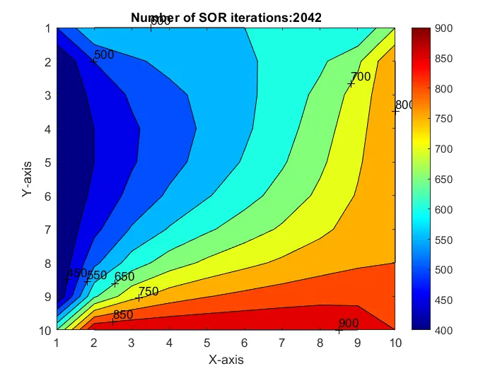
    title(sprintf('Number of SOR iterations:%d',iter));
    pause(0.03)
end
PLOT
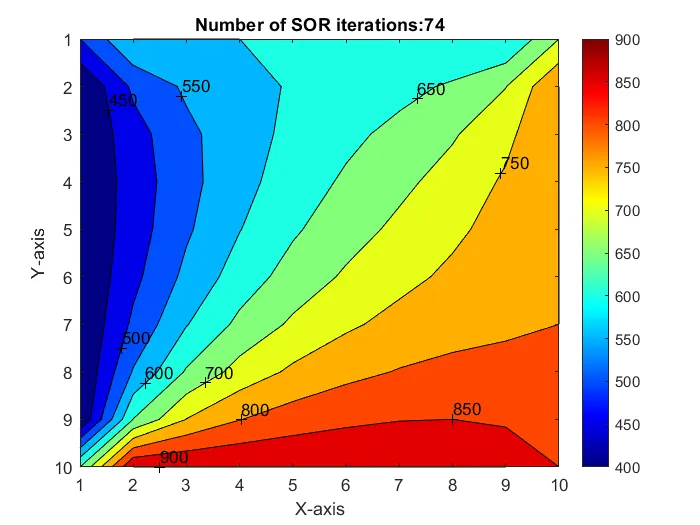
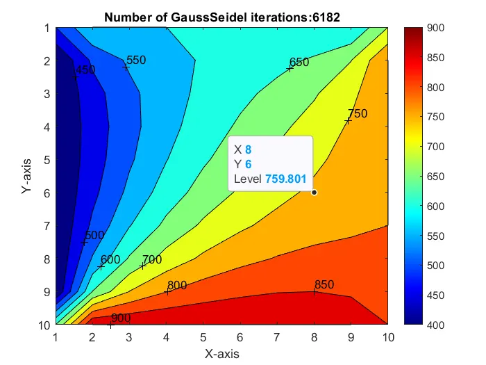
The plots show temperature contours in the x-y domain. As inferred from the plots, we can conclude that no.of iterations required for the Jacobi method is more i.e.
No.of Jacobi iterations>No of Gauss-Seidel iterations>No of SOR iterations
TRANSIENT CASE
For the transient case, two approaches exist-Implicit and explicit.
Implicit approach involves calculating values for the current timestep involving parameters at the current timestep.
Explicit approach involves calculating values for the current timestep involving parameters from the previous timestep.
Explicit Approach
The unsteady 2-D conduction equation is `(delT)/(delt)=alpha((del^2T)/(delx^2)+(del^2T)/(dely^2))`
Discretising the above equation,
`(underset(p)(overset(n+1)(T)) - underset(p)(overset(n)(T)))/(Deltax) =alpha(overset(n)((underset(L)(T)-2*underset(P)(T)+underset(R)(T))/(Deltax^2) +(underset(B)(T)-2*underset(P)(T)+underset(T)(T))/(Deltay^2)))`
The solution becomes
`underset(p)(overset(n+1)(T) =underset(p)(overset(n)(T))+underset(1)(k)(underset(L)(T)-2*underset(P)(T)+underset(R)(T))+underset(2)(k)(underset(T)(T)-2*underset(P)(T)+underset(B)(T))`
where the value to be calculated at the timestep n+1 is obtained from the values which are calculated at timestep n.
where `underset(1)(k)=alpha((Deltat)/(Deltax^2)) ; underset(2)(k)=alpha((Deltat)/(Deltay^2))`
The program is solved for three iterative solvers-GaussSeidel,Jacobi and SuccessiveOverRelaxation methods by assuming suitable values.
JACOBI method-Explicit Scheme
%to solve the unsteady conduction equation dT/dt=k(d^2T/dx^2 +d^2T/dy^2)

%Initial values
n_x=10;  %no of divisions along x direction
n_y=10;  %no of divisions along y direction
x=linspace(1,n_x,10);
y=linspace(1,n_y,10);
dx=x(2)-x(1);   %grid dimension in x direction
dy=y(2)-y(1);   %grid dimension in y direction

%Initializing and Boundary Conditions
T=300*ones(n_x,n_y);
T(1,2:n_x-1)=600;         %Temperature at the top is 600K
T(10,2:n_x-1)=900;        %Temperature at the bottom is 900K
T(2:n_y-1,1)=400;         %Temperature on the left side is 400K
T(2:n_y-1,10)=800;        %Temperature on the right side is 800K

%Temperature at corners
T(1,1)=500;
T(1,10)=700;
T(10,1)=650;
T(10,10)=850;
T_old=T;
T_initial=T;    %temperature at timestep n

%Solving
%Consider explicit
dt=0.02;
t=0.15; q=0.3;
k1=q*dt/(dx^2);
k2=q*dt/(dy^2);
n_t=t/dt;    %no of timesteps
T(10,1)=650;
T(10,10)=850;
T_old=T;
T_initial=T;    %temperature at timestep n

%Solving
%Consider explicit
dt=0.02;
t=0.15; q=0.3;
k1=q*dt/(dx^2);
k2=q*dt/(dy^2);
n_t=t/dt;    %no of timesteps
tolerance=1e-4;
iter=1;

%refer notes to check about term 1. term1=(1+2k1+2k2)^-1    %Jacobi
%Method
tic
for a=1:n_t

    error=10e5;
    T_initial=T;
    while error>tolerance
        for i=2:n_x-1
            for j=2:n_y-1
                T(i,j)=(T_old(i,j)*term1)+(k1*(T_old(i-1,j)+T_old(i+1,j)-2*T_old(i,j)))+(k2*(T_old(i,j+1)+T_old(i,j-1)-2*T_old(i,j)));
            end
        end
        iter=iter+1;
        error=max(max(abs(T_old-T)));
        T_old=T;
        figure(1)
        contourf(x,y,T)
        clabel(contourf(x,y,T))
        colorbar
        colormap(jet)
        set(gca,'ydir','reverse')
        xlabel('X-axis');
        ylabel('Y-axis');
        title(sprintf('Number of Jacobi iterations:%d',iter));

    end
    T_initial=T;
end
iter_time=toc;
GAUSS Seidel-Explicit
%to solve the unsteady conduction equation dT/dt=k(d^2T/dx^2 +d^2T/dy^2)

%Initial values
n_x=10;  %no of divisions along x direction
n_y=10;  %no of divisions along y direction
x=linspace(1,n_x,10);
y=linspace(1,n_y,10);
dx=x(2)-x(1);   %grid dimension in x direction
dy=y(2)-y(1);   %grid dimension in y direction

%Initializing and Boundary Conditions
T=300*ones(n_x,n_y);
T(1,2:n_x-1)=600;         %Temperature at the top is 600K
T(10,2:n_x-1)=900;        %Temperature at the bottom is 900K
T(2:n_y-1,1)=400;         %Temperature on the left side is 400K
T(2:n_y-1,10)=800;        %Temperature on the right side is 800K

%Temperature at corners
T(1,1)=500;
T(1,10)=700;
T(10,1)=650;
T(10,10)=850;
T_old=T;
T_initial=T;    %temperature at timestep n

%Solving
%Consider explicit
dt=0.02;
t=0.15; q=0.3;
k1=q*dt/(dx^2);
k2=q*dt/(dy^2);
n_t=t/dt;    %no of timesteps
tolerance=1e-4;
iter=1;

%refer notes to check about term 1. term1=(1+2k1+2k2)^-1    %Jacobi
%Method
tic
for a=1:n_t

    error=10e5;
    T_initial=T;
    while error>tolerance
        for i=2:n_x-1
            for j=2:n_y-1
                T(i,j)=T(i,j)+(k1*(T(i-1,j)+T_old(i+1,j)-2*T_old(i,j)))+(k2*(T_old(i,j+1)+T(i,j-1)-2*T_old(i,j)));
            end
        end
        iter=iter+1;
        error=max(max(abs(T_old-T)));
        T_old=T;
        figure(1)
        contourf(x,y,T)
        clabel(contourf(x,y,T))
        colorbar
        colormap(jet)
        set(gca,'ydir','reverse')
        xlabel('X-axis');
        ylabel('Y-axis');
        title(sprintf('Number of GaussSeidel iterations:%d',iter));
        pause(0.03)
    end
    T_initial=T;
end
iter_time=toc;
The plot for the GaussSeidel method
Implicit Approach
Recalling that the unsteady 2-D conduction equation is `(delT)/(delt)=alpha((del^2T)/(delx^2)+(del^2T)/(dely^2))`
Discretising the above equation,
`(underset(p)(overset(n+1)(T)) - underset(p)(overset(n)(T)))/(Deltax) =alpha(overset(n+1)((underset(L)(T)-2*underset(P)(T)+underset(R)(T))/(Deltax^2) +(underset(B)(T)-2*underset(P)(T)+underset(T)(T))/(Deltay^2)))`
The solution becomes
`underset(p)(overset(n+1)(T))=(1/(2*underset(1)k +2*underset(2)k +1))(underset(p)(overset(n)(T))+underset(1)koverset(n+1)((underset(L)(T)+underset(R)(T)))+underset(2)(k)overset(n+1)((underset(T)(T)+underset(B)(T))))`
where
`underset(1)(k)=alpha((Deltat)/(Deltax^2)) ; underset(2)(k)=alpha((Deltat)/(Deltay^2))`
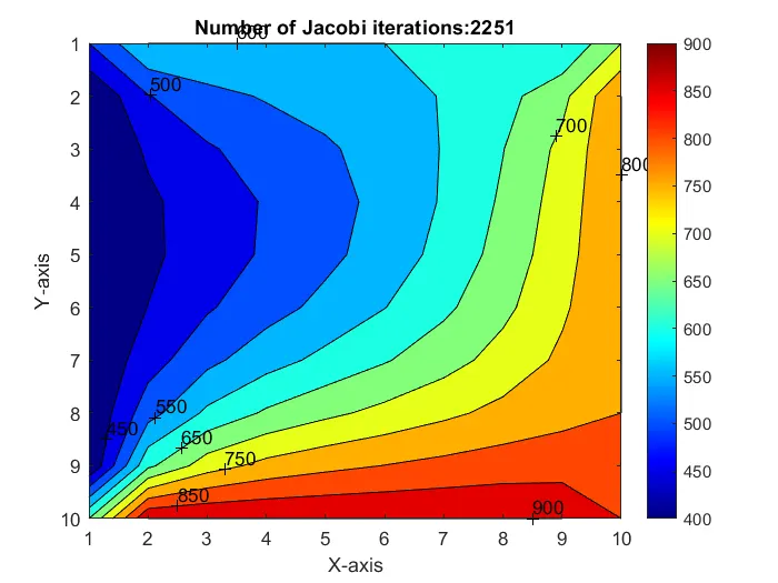
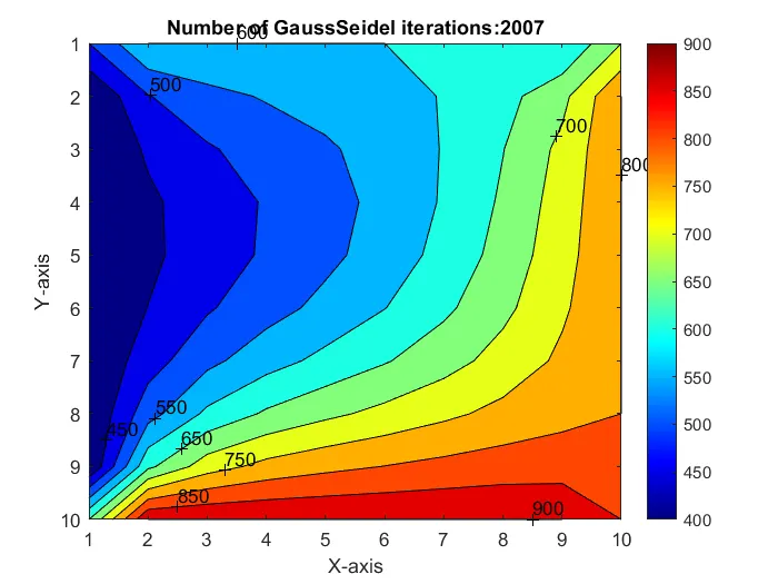
Solving the implicit form using the three iterative solvers,we get three different plots.
JACOBI METHOD
%to solve the unsteady conduction equation dT/dt=k(d^2T/dx^2 +d^2T/dy^2)

%Initial values
n_x=10;  %no of divisions along x direction
n_y=10;  %no of divisions along y direction
x=linspace(1,n_x,10);
y=linspace(1,n_y,10);
dx=x(2)-x(1);   %grid dimension in x direction
dy=y(2)-y(1);   %grid dimension in y direction

%Initializing and Boundary Conditions
T=300*ones(n_x,n_y);
T(1,2:n_x-1)=600;         %Temperature at the top is 600K
T(10,2:n_x-1)=900;        %Temperature at the bottom is 900K
T(2:n_y-1,1)=400;         %Temperature on the left side is 400K
T(2:n_y-1,10)=800;        %Temperature on the right side is 800K

%Temperature at corners
T(1,1)=500;
T(1,10)=700;
T(10,1)=650;
T(10,10)=850;
T_old=T;
T_previous=T;         %temperature at timestep n

%Solving
%Consider Implicit
dt=0.01;
t=5; q=1.4;
k1=q*dt/(dx^2);
k2=q*dt/(dy^2);
n_t=t/dt;    %no of timesteps
tolerance=1e-4;
iter=1;
w=1.2;%refer notes to check about term 1. term1=(1+2k1+2k2)^-1    %Jacobi
%Method
term1=1/(1+ 2*k1 +2*k2);
tic
for a=1:n_t

    error=10e4;
    while error>tolerance
        for i=2:n_x-1
            for j=2:n_y-1
                T(i,j)=(T_previous(i,j)*term1)+ (term1*k1*((T_old(i-1,j) +T_old(i+1,j))) + term1*k2*(T_old(i,j+1)+T_old(i,j-1)));
            end
        end
        iter=iter+1;
        error=max(max(abs(T_old-T)));
        T_old=T;
    end
    T_previous=T;
end
iter_time=toc;
        figure(1)
        contourf(x,y,T)
        clabel(contourf(x,y,T))
        colorbar
        colormap(jet)
        set(gca,'ydir','reverse')
        xlabel('X-axis');
        ylabel('Y-axis');
        title(sprintf('Number of Jacobi iterations:%d',iter));
PLOT
GaussSeidel
%to solve the unsteady conduction equation dT/dt=k(d^2T/dx^2 +d^2T/dy^2)

%Initial values
n_x=10;  %no of divisions along x direction
n_y=10;  %no of divisions along y direction
x=linspace(1,n_x,10);
y=linspace(1,n_y,10);
dx=x(2)-x(1);   %grid dimension in x direction
dy=y(2)-y(1);   %grid dimension in y direction

%Initializing and Boundary Conditions
T=300*ones(n_x,n_y);
T(1,2:n_x-1)=600;         %Temperature at the top is 600K
T(10,2:n_x-1)=900;        %Temperature at the bottom is 900K
T(2:n_y-1,1)=400;         %Temperature on the left side is 400K
T(2:n_y-1,10)=800;        %Temperature on the right side is 800K

%Temperature at corners
T(1,1)=500;
T(1,10)=700;
T(10,1)=650;
T(10,10)=850;
T_old=T;
T_previous=T;         %temperature at timestep n

%Solving
%Consider Implicit
dt=0.01;
t=5; q=1.4;
k1=q*dt/(dx^2);
k2=q*dt/(dy^2);
n_t=t/dt;    %no of timesteps
tolerance=1e-4;
iter=1;
w=1.2;%refer notes to check about term 1. term1=(1+2k1+2k2)^-1    %Jacobi
%Method
term1=1/(1+ 2*k1 +2*k2);
tic
for a=1:n_t

    error=10e4;
    while error>tolerance
        for i=2:n_x-1
            for j=2:n_y-1
                %GaussSeidel
                T(i,j)=(T_previous(i,j)*term1)+ (term1*k1*((T(i-1,j) +T_old(i+1,j))) + term1*k2*(T_old(i,j+1)+T(i,j-1)));
end
        end
        iter=iter+1;
        error=max(max(abs(T_old-T)));
        T_old=T;
    end
    T_previous=T;
end
iter_time=toc;
        figure(1)
        contourf(x,y,T)
        clabel(contourf(x,y,T))
        colorbar
        colormap(jet)
        set(gca,'ydir','reverse')
        xlabel('X-axis');
        ylabel('Y-axis');
        title(sprintf('Number of GaussSeidel iterations:%d',iter));
PLOT
Successive-OverRelaxation
%to solve the unsteady conduction equation dT/dt=k(d^2T/dx^2 +d^2T/dy^2)

%Initial values
n_x=10;  %no of divisions along x direction
n_y=10;  %no of divisions along y direction
x=linspace(1,n_x,10);
y=linspace(1,n_y,10);
dx=x(2)-x(1);   %grid dimension in x direction
dy=y(2)-y(1);   %grid dimension in y direction

%Initializing and Boundary Conditions
T=300*ones(n_x,n_y);
T(1,2:n_x-1)=600;         %Temperature at the top is 600K
T(10,2:n_x-1)=900;        %Temperature at the bottom is 900K
T(2:n_y-1,1)=400;         %Temperature on the left side is 400K
T(2:n_y-1,10)=800;        %Temperature on the right side is 800K

%Temperature at corners
T(1,1)=500;
T(1,10)=700;
T(10,1)=650;
T(10,10)=850;
T_old=T;
T_previous=T;         %temperature at timestep n

%Solving
%Consider Implicit
dt=0.01;
t=5; q=1.4;
k1=q*dt/(dx^2);
k2=q*dt/(dy^2);
n_t=t/dt;    %no of timesteps
tolerance=1e-4;
iter=1;
w=1.2;%refer notes to check about term 1. term1=(1+2k1+2k2)^-1    %Jacobi
%Method
term1=1/(1+ 2*k1 +2*k2);
tic
for a=1:n_t

    error=10e4;
    while error>tolerance
        for i=2:n_x-1
            for j=2:n_y-1
                %SOR
                termA=T(i-1,j)+T_old(i+1,j);
                termB=T(i,j-1)+T_old(i,j+1);
                T(i,j)=T_previous(i,j)*(1-w) + w*term1*(T_previous(i,j)+k1*termA +k2*termB);

            end
        end
        iter=iter+1;
        error=max(max(abs(T_old-T)));
        T_old=T;

    end
    T_previous=T;
end
iter_time=toc;
        figure(1)
        contourf(x,y,T)
        clabel(contourf(x,y,T))
        colorbar
        colormap(jet)
        set(gca,'ydir','reverse')
        xlabel('X-axis');
        ylabel('Y-axis');
        title(sprintf('Number of SOR iterations:%d',iter));
PLOT
RESULTS AND DISCUSSIONS
From the above plots, we can infer that Jacobi Iteration requires a large number of iterations compared to Gauss-Seidel and SOR.