Week 4 - CHT Analysis on Exhaust port

Challenge:

In this challenge, we are going to conduct a CHT(aka conjugate heat transfer) analysis in an exhaust port in Ansys Fluent. Here, we will try to explain what is Y+ and what are its use, calculate the surface heat transfer coefficient on the internal solid surface and show the velocity.

CHT(Conjugate Heat Transfer):

Conjugate heat transfer is a type of heat transfer analysis between solids and fluid(s). This type of heat transfer includes both convection (between fluids) and conductive (between solids) heat transfer, as well as both forced and natural convection. Common applications and use cases of this thermal simulation type include electronics cooling, heat exchangers, industrial machinery,etc.

In most cases, heat transfer in solids, if only due to conduction is given by fourier's law of heat conduction which describes heat flux as `q=-knablaT`, whereas for a time-dependent problem, the temperature field in an immobile solid verifies the following form of the heat equation:

`rho*underset(p)(C)*(delT)/(delt)=nabla.(knablaT)+Q`

In a fluid, due to the fluid motion, three contributions to the heat equation are included:

1. The transport of fluid implies energy transport too, which appears in the heat equation as the convective contribution. Depending on the thermal properties on the fluid and on the flow regime, either the convective or the conductive heat transfer can dominate.
2. The viscous effects of the fluid flow produce fluid heating. This term is often neglected, nevertheless, its contribution is noticeable for fast flow in viscous fluids.
3. As soon as a fluid density is temperature-dependent, a pressure work term contributes to the heat equation. This accounts for the well-known effect that, for example, compressing air produces heat.

Heat transfer in fluids and solids can also be combined to minimize heat losses in various devices. Because most gases (especially at low pressure) have small thermal conductivities, they can be used as thermal insulators. In areas which involve cooling of components like turbine blades and transfer of heats across media, CHT is necessary to accurately model the system.

Procedure:

The process involves importing the cad file in spaceclaim, then certain modifications are done to the CAD file so that it is perfect for meshing. THhis is followed by setting up the solver and applying flow turbulence models, boundary conditions etc. Once these are done, the solution is run for a certain number of iterations until it converges. Then post processing is performed where we get contours of velocity, temperature etc in the pipe and at a planar section.

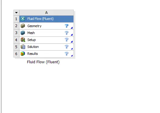
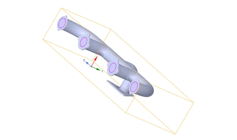
Drag and drop fluent module into the project schematic window. The first step is to extract fluid volume from the geometry. Next step is to share the topology and make sure that the surfaces are shared. Once the process is done, it will look something like this.

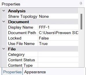
Turn on the share topology

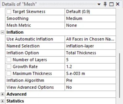
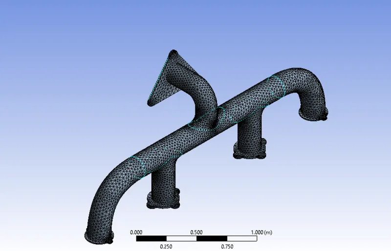
The next step is to mesh the geometry. This involves meshing and refining and adding inflation layers to the fluid solid interface so as to capture convection coefficient.

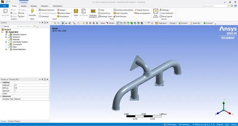
Select inflation option and give maximum thickness value of 5mm. Once done, the mesh should look something like this:

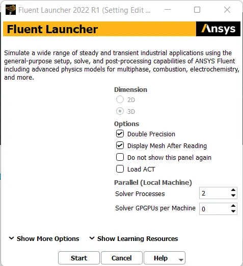
Once meshing is done, update the mesh and close it. Open Fluent setup

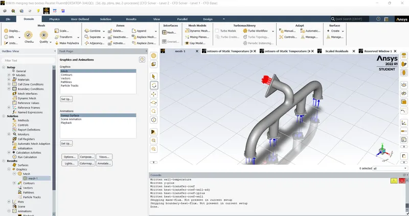
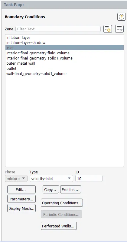
Mention the type of viscous model and solver used. Next mention the boundary conditions (inlet velocity and inlet temperature are 5 m/s and 700 K respectively). To visualise the solution, create an animation playback so as to view the runtime of the solution as a video file and save it.

The solution remains almost converged for a set of iterations and post processing is carried out by CFD Post. In CFD post, we plot contours of velocity variation along a pipe section at the outlet(say) and calculate temperature contours and heat transfer coefficient.

With inflation layer

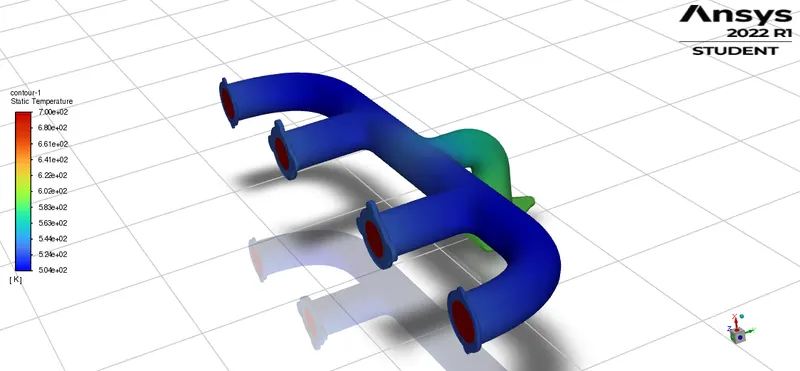
Contours of temperature over the entire exhaust port

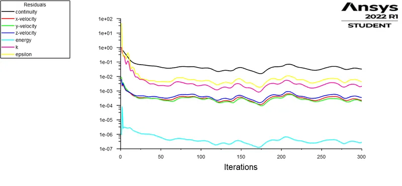
Convergence of the solution

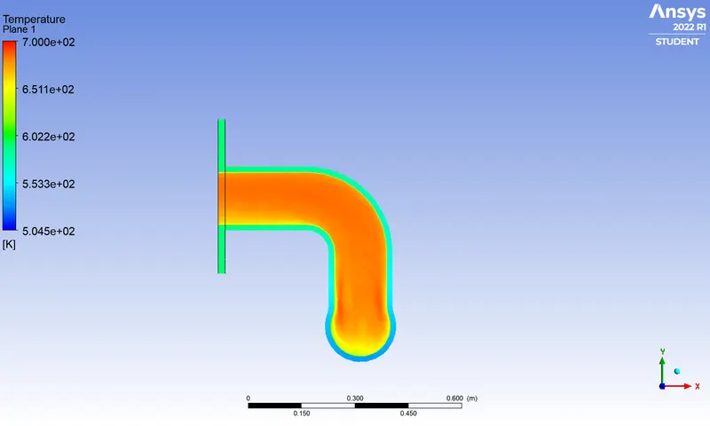
Temperature contours over the outlet cross section

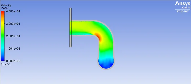
Velocity contours over the outlet cross section

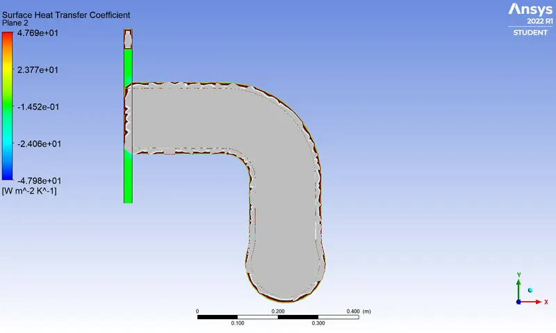
Heat transfer coefficient over the cross section of the pipe

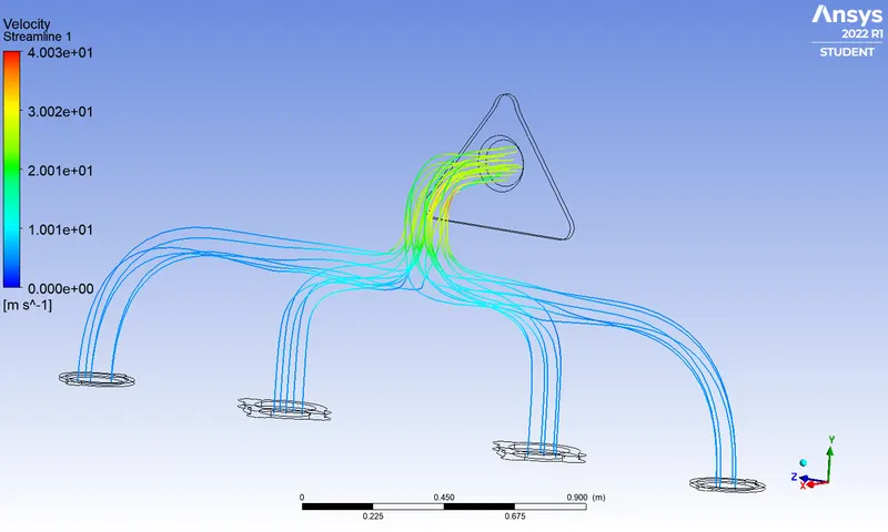
Streamlines plotted in the port

The same procedure mentioned above is repeated for a case without inflation layer.

Without inflation layer

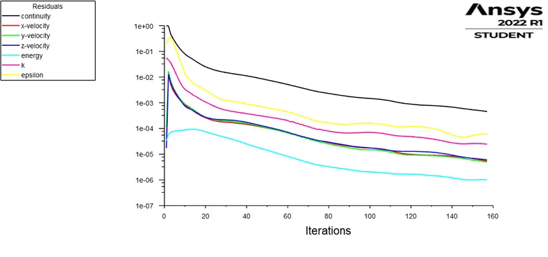
Convergence of the solution

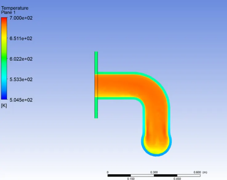
Temperature contours at a cross-section of the pipe

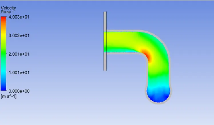
Velocity contours at a cross section of the pipe

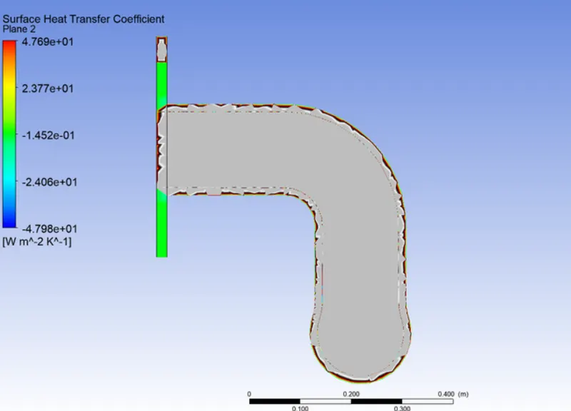
Heat transfer coefficient over the cross section of the pipe

The key difference in the above two cases are that the number of iterations taken to converge without providing inflation layers is very less. There is little to no difference between providing inflation layers and without inflation layers.

Y+ is the non dimensional distance normal to the wall. In a turbulent boundary layer, there are three subzones-viscous sublayer, buffer region and log-law region.

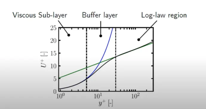
In the viscous sublayer, y+ <5

In the log-law region 30<y+<200

Since the mesh refinement is limited in the ansys version, we use k-epsilon model which has y+ value in the range of 30-300.

Y+ calculation

CS Area of pipe=0.0217 sq m

radius of the pipe=0.0831 m

Therefore,`Re=(rho*V*D)/mu` =0.5687*`10^5`

`underset(f)(C)=0.059/(Re)^.2`=0.006605

Wall shear stress `underset(w)(tau)=.5*rho*V^2*underset(f)(C)`=0.1011

`underset(t)(U)=sqrt(underset(w)(tau)/rho)`=.2873 m/s

Assuming first cell height as 0.005 m,

then Y+=98.3 for this model. which lies in the range. To refine it further, make sure that the value of Y+ remains closer to 1. To achieve this, we have to use k-omega model.

Comparing theoretical data with computed data:

Nusselt's number is given by `Nu=0.023*Re^0.75*Pr^0.4` for turbulent flow through a pipe

Calculating, Nu comes around 75.476

But `Nu=hL/k implies h=Nk/L`

`impliesh=10.899W/(m^2K)`

Computed average value=11.8124 `W/(m^2K)`

If the mesh is refined more, the accuracy of the solution will be better.

Conclusion:

Thus the setting up of the exhaust port in Fluent has been understood and sufficient analysis is carried out.

Also we learnt about the following details as well:

->Geometry preparation in Spaceclaim - Extra edges, Fluid volume extraction, share topology

->Introduction to CHT simulation

->High-temperature concentration zone prediction

->Comparison between the solver models for accurate results