Project 1- Creating your own OpenFOAM solver
Creating your own OpenFOAM solver
In this challenge, the objective is to create a custom OpenFOAM software by modifying some details in the codes and in the files.
At first, the solver is copied from ~applications/solvers/incompressible/icoFoam and the folder is renamed as scalarFoam. Once done, rename the code as scalarFoam.C
Changes in scalarFoam.C
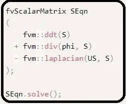
Below is the scalarFoam.C code that has been modified by adding terms for the scalar transport terms as shown below:
/*---------------------------------------------------------------------------*\
  =========                 |
  \\      /  F ield         | OpenFOAM: The Open Source CFD Toolbox
   \\    /   O peration     |
    \\  /    A nd           | www.openfoam.com
     \\/     M anipulation  |
-------------------------------------------------------------------------------
    Copyright (C) 2011-2016 OpenFOAM Foundation
    Copyright (C) 2019 OpenCFD Ltd.
-------------------------------------------------------------------------------
License
    This file is part of OpenFOAM.

    OpenFOAM is free software: you can redistribute it and/or modify it
    under the terms of the GNU General Public License as published by
    the Free Software Foundation, either version 3 of the License, or
    (at your option) any later version.

    OpenFOAM is distributed in the hope that it will be useful, but WITHOUT
    ANY WARRANTY; without even the implied warranty of MERCHANTABILITY or
    FITNESS FOR A PARTICULAR PURPOSE.  See the GNU General Public License
    for more details.

    You should have received a copy of the GNU General Public License
    along with OpenFOAM.  If not, see <http://www.gnu.org/licenses/>.

Application
    icoFoam

Group
    grpIncompressibleSolvers

Description
    Transient solver for incompressible, laminar flow of Newtonian fluids.

    \heading Solver details
    The solver uses the PISO algorithm to solve the continuity equation:

        \f[
            \div \vec{U} = 0
        \f]

    and momentum equation:

        \f[
            \ddt{\vec{U}}
          + \div \left( \vec{U} \vec{U} \right)
          - \div \left(\nu \grad \vec{U} \right)
          = - \grad p
        \f]

    Where:
    \vartable
        \vec{U} | Velocity
        p       | Pressure
    \endvartable

    \heading Required fields
    \plaintable
        U       | Velocity [m/s]
        p       | Kinematic pressure, p/rho [m2/s2]
    \endplaintable

\*---------------------------------------------------------------------------*/

#include "fvCFD.H"
#include "pisoControl.H"

// * * * * * * * * * * * * * * * * * * * * * * * * * * * * * * * * * * * * * //

int main(int argc, char *argv[])
{
    argList::addNote
    (
        "Transient solver for incompressible, laminar flow"
        " of Newtonian fluids."
    );

    #include "postProcess.H"

    #include "addCheckCaseOptions.H"
    #include "setRootCaseLists.H"
    #include "createTime.H"
    #include "createMesh.H"

    pisoControl piso(mesh);

    #include "createFields.H"
    #include "initContinuityErrs.H"

    // * * * * * * * * * * * * * * * * * * * * * * * * * * * * * * * * * * * //

    Info<< "\nStarting time loop\n" << endl;

    while (runTime.loop())
    {
        Info<< "Time = " << runTime.timeName() << nl << endl;

        #include "CourantNo.H"

        // Momentum predictor

        fvVectorMatrix UEqn
        (
            fvm::ddt(U)
          + fvm::div(phi, U)
          - fvm::laplacian(nu, U)
        );

        if (piso.momentumPredictor())
        {
            solve(UEqn == -fvc::grad(p));
        }

        // --- PISO loop
        while (piso.correct())
        {
            volScalarField rAU(1.0/UEqn.A());
            volVectorField HbyA(constrainHbyA(rAU*UEqn.H(), U, p));
            surfaceScalarField phiHbyA
            (
                "phiHbyA",
                fvc::flux(HbyA)
              + fvc::interpolate(rAU)*fvc::ddtCorr(U, phi)
            );

            adjustPhi(phiHbyA, U, p);

            // Update the pressure BCs to ensure flux consistency
            constrainPressure(p, U, phiHbyA, rAU);

            // Non-orthogonal pressure corrector loop
            while (piso.correctNonOrthogonal())
            {
                // Pressure corrector

                fvScalarMatrix pEqn
                (
                    fvm::laplacian(rAU, p) == fvc::div(phiHbyA)
                );

                pEqn.setReference(pRefCell, pRefValue);

                pEqn.solve(mesh.solver(p.select(piso.finalInnerIter())));

                if (piso.finalNonOrthogonalIter())
                {
                    phi = phiHbyA - pEqn.flux();
                }
            }

            #include "continuityErrs.H"

            U = HbyA - rAU*fvc::grad(p);
            U.correctBoundaryConditions();

        }

        fvScalarMatrix SEqn
        (
            fvm::ddt(S)
          + fvm::div(phi, S)
          - fvm::laplacian(US, S)
        );

        SEqn.solve();

        runTime.write();

        runTime.printExecutionTime(Info);
    }

    Info<< "End\n" << endl;

    return 0;
}


// ************************************************************************* //
where US is the viscosity term in the scalar transport equation(eventhough it doesnt have any, but for the sake of simplicity).
Once done, we have to write an IOobject for our scalar property S
Changing createFields.H
Just like there is a viscosity term "nu" , we add the viscosity term for the scalar equation "SU".
We also add a scalarField for S just as in the same way for p.
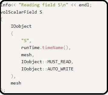
This is shown below:
Info<< "Reading transportProperties\n" << endl;

IOdictionary transportProperties
(
    IOobject
    (
        "transportProperties",
        runTime.constant(),
        mesh,
        IOobject::MUST_READ_IF_MODIFIED,
        IOobject::NO_WRITE
    )
);

dimensionedScalar nu
(
    "nu",
    dimViscosity,
    transportProperties
);

dimensionedScalar US
(
    "SU",
    dimViscosity,
    transportProperties
);

Info<< "Reading field p\n" << endl;
volScalarField p
(
    IOobject
    (
        "p",
        runTime.timeName(),
        mesh,
        IOobject::MUST_READ,
        IOobject::AUTO_WRITE
    ),
    mesh
);


Info<< "Reading field U\n" << endl;
volVectorField U
(
    IOobject
    (
        "U",
        runTime.timeName(),
        mesh,
        IOobject::MUST_READ,
        IOobject::AUTO_WRITE
    ),
    mesh
);

Info<< "Reading field S\n" << endl;
volScalarField S
(
    IOobject
    (
        "S",
        runTime.timeName(),
        mesh,
        IOobject::MUST_READ,
        IOobject::AUTO_WRITE
    ),
    mesh
);


#include "createPhi.H"


label pRefCell = 0;
scalar pRefValue = 0.0;
setRefCell(p, mesh.solutionDict().subDict("PISO"), pRefCell, pRefValue);
mesh.setFluxRequired(p.name());
Changing Make files and options
The next step is to make changes to the make files. Go to Make->files and rename the code to scalarFoam.C and the others as follows:
scalarFoam.C

EXE = $(FOAM_USER_APPBIN)/scalarFoam
The Make->options look something like this
EXE_INC = \
    -I$(LIB_SRC)/finiteVolume/lnInclude \
    -I$(LIB_SRC)/meshTools/lnInclude

EXE_LIBS = \
    -lfiniteVolume \
    -lmeshTools
Once done, compile using wmake to check whether solver runs.
Changing 0 files
Once done with make, the next step is to copy a case file($FOAM_TUTORIALS/incompressible/icoFoam/cavity) and using the scalarFoam as the solver.
First lets create a copy of p file and save it as S file. Here, we consider S as temperature by specifying the value of temperature at the boundaries, as shown below:
/*--------------------------------*- C++ -*----------------------------------*\
| =========                 |                                                 |
| \\      /  F ield         | OpenFOAM: The Open Source CFD Toolbox           |
|  \\    /   O peration     | Version:  v2206                                 |
|   \\  /    A nd           | Website:  www.openfoam.com                      |
|    \\/     M anipulation  |                                                 |
\*---------------------------------------------------------------------------*/
FoamFile
{
    version     2.0;
    format      ascii;
    class       volScalarField;
    object      p;
}
// * * * * * * * * * * * * * * * * * * * * * * * * * * * * * * * * * * * * * //

dimensions      [0 0 0 1 0 0 0];

internalField   uniform 400;

boundaryField
{
    movingWall
    {
        type            fixedValue;
	  value		uniform 500;
    }

    fixedWalls
    {
        type            fixedValue;
	  value		uniform 300;
    }

    frontAndBack
    {
        type            empty;
    }
}


// ************************************************************************* //
Once done, the next step is to update transport properties. Specify the value of viscosity "SU" in the transportProperties file.
/*--------------------------------*- C++ -*----------------------------------*\
| =========                 |                                                 |
| \\      /  F ield         | OpenFOAM: The Open Source CFD Toolbox           |
|  \\    /   O peration     | Version:  v2206                                 |
|   \\  /    A nd           | Website:  www.openfoam.com                      |
|    \\/     M anipulation  |                                                 |
\*---------------------------------------------------------------------------*/
FoamFile
{
    version     2.0;
    format      ascii;
    class       dictionary;
    object      transportProperties;
}
// * * * * * * * * * * * * * * * * * * * * * * * * * * * * * * * * * * * * * //

nu              0.01;
SU		    0.01;


// ************************************************************************* //
Once done, go to controlDict and change the name of the solver to scalarFoam. This will make sure that our solver is executed.
/*--------------------------------*- C++ -*----------------------------------*\
| =========                 |                                                 |
| \\      /  F ield         | OpenFOAM: The Open Source CFD Toolbox           |
|  \\    /   O peration     | Version:  v2206                                 |
|   \\  /    A nd           | Website:  www.openfoam.com                      |
|    \\/     M anipulation  |                                                 |
\*---------------------------------------------------------------------------*/
FoamFile
{
    version     2.0;
    format      ascii;
    class       dictionary;
    object      controlDict;
}
// * * * * * * * * * * * * * * * * * * * * * * * * * * * * * * * * * * * * * //

application     scalarFoam;

startFrom       startTime;

startTime       0;

stopAt          endTime;

endTime         0.5;

deltaT          0.005;

writeControl    timeStep;

writeInterval   20;

purgeWrite      0;

writeFormat     ascii;

writePrecision  6;

writeCompression off;

timeFormat      general;

timePrecision   6;

runTimeModifiable true;


// ************************************************************************* //
Changing interpolation schemes and solvers
The next step is to implement interpolation schemes for the convective term(`\grad.SU`) in the file fvSchemes. We specify Gauss linear as the interpolation scheme.
/*--------------------------------*- C++ -*----------------------------------*\
| =========                 |                                                 |
| \\      /  F ield         | OpenFOAM: The Open Source CFD Toolbox           |
|  \\    /   O peration     | Version:  v2206                                 |
|   \\  /    A nd           | Website:  www.openfoam.com                      |
|    \\/     M anipulation  |                                                 |
\*---------------------------------------------------------------------------*/
FoamFile
{
    version     2.0;
    format      ascii;
    class       dictionary;
    object      fvSchemes;
}
// * * * * * * * * * * * * * * * * * * * * * * * * * * * * * * * * * * * * * //

ddtSchemes
{
    default         Euler;
}

gradSchemes
{
    default         Gauss linear;
    grad(p)         Gauss linear;
}

divSchemes
{
    default         none;
    div(phi,U)      Gauss linear;
    div(phi,S)	  Gauss linear;
}

laplacianSchemes
{
    default         Gauss linear orthogonal;
}

interpolationSchemes
{
    default         linear;
}

snGradSchemes
{
    default         orthogonal;
}


// ************************************************************************* //
In the file fvSolution, copy the contents of p and paste it as S and specify the solvers and save it. If we use the same solver as that for p, we will get an error due to asymmetry of the matrix.
/*--------------------------------*- C++ -*----------------------------------*\
| =========                 |                                                 |
| \\      /  F ield         | OpenFOAM: The Open Source CFD Toolbox           |
|  \\    /   O peration     | Version:  v2206                                 |
|   \\  /    A nd           | Website:  www.openfoam.com                      |
|    \\/     M anipulation  |                                                 |
\*---------------------------------------------------------------------------*/
FoamFile
{
    version     2.0;
    format      ascii;
    class       dictionary;
    object      fvSolution;
}
// * * * * * * * * * * * * * * * * * * * * * * * * * * * * * * * * * * * * * //

solvers
{
    p
    {
        solver          PCG;
        preconditioner  DIC;
        tolerance       1e-06;
        relTol          0.05;
    }

    pFinal
    {
        $p;
        relTol          0;
    }

    U
    {
        solver          smoothSolver;
        smoother        symGaussSeidel;
        tolerance       1e-05;
        relTol          0;
    }

    S
    {
        solver          PBiCG;
        preconditioner  DILU;
        tolerance       1e-06;
        relTol          0.05;
    }
}

PISO
{
    nCorrectors     2;
    nNonOrthogonalCorrectors 0;
    pRefCell        0;
    pRefValue       0;
}


// ************************************************************************* //
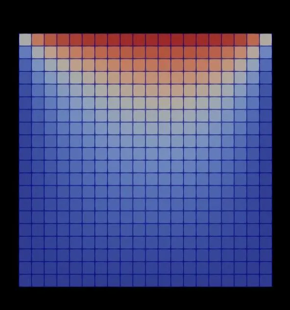
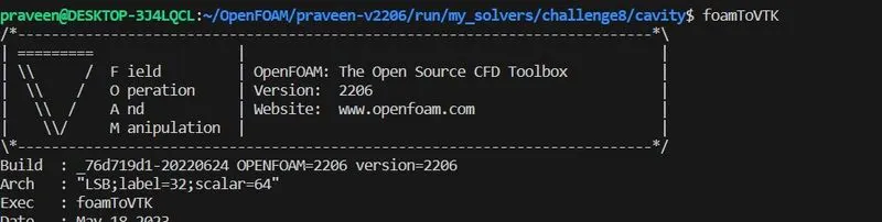
Once done, run blockMesh and checkMesh and scalarFoam and the results are shown below. Also type foamToVTK so as to open the files in PARAVIEW.
We can also see that our solver is solving for S, our scalar property.
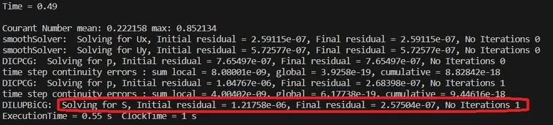
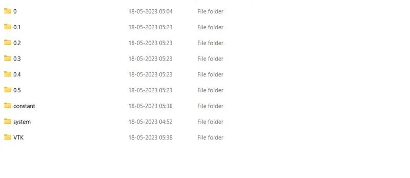
As you can see above, open the VTK folder and open the file in paraVIEW so as to see the simulation.