Week 9 - Senstivity Analysis Assignment

Senstivity Analysis Assignment

Aim

In this experiment, we will be working on a source code provided in the video by doing minor changes like:

-> writing a code that takes all the reactions from the GRI mechanism and calculating 10 most sensitive reactions

-> The sensitivity parameter created should be with respect to the Temperature

-> To consider the initial conditions as shown in the video

Theory

-> Parameters in the heat conduction equation are frequently modeled as temperature dependent.

-> Thermal conductivity, volumetric heat capacity, convection coefficient, emmisivity and volumetric source terms are parameters that may depends on temperature.

-> Many applications, such as parameter estimations, optical experimental design, optimization and uncertainity analysis, require sensitivity to the parameters describing temperature dependent proparties.

-> A general procedure to compute the sensitivity of the temperature field to model parameters for nonlinear heat conduction is studied.

-> Parameters are modeled as arbitrary function of temperature. Sensitivity equations are implimented is an unstructured grid, element based numerical solver.

-> The objectives of this study are to describe the methodology to derive sensitivity equation for the temperature-dependent parameters and present demonstrations calculations.

-> In addition to a verification problem, the design of an experiment to estimate temperature variable thermal proparties is discussed.

-> Sensitivity analysis is a method for predicting the outcome of a decision if a situation turns out tobe different compared to the key predictions.

-> It helps in assessing the riskiness of a strategy. Helps in identifying how dependent the output is on a particular input value.

-> The various techniques widely applied include: Differential sensitivity analysis, One at a time sensitivity measures, Factorial analysis, Correlation analysis, Regression analysis, Subjective sensitivity analysis, etc.

-> One of the key applications of sensitivity analysis is in the utilizations of models by manegers and decision makers.

-> All the content needed for the decision model can be fully utilized only through the repeated applications of sensitivity analysis.

-> It helps decision analysts to understand the uncertainities, pros and cons with the limitations and scope of a decision model.

-> The key application of sensitivity analysis is to indicate the sensitivity of simulation to uncertainities in the input values of the model.

-> This helps in decision making. Sensitivity analysis is a method for predicting the outcome of a decision if a situation turns out tobe different compared to the key predictions.

-> It helps in assessing the riskiness of a strategy

-> It helps in identifying how dependent the output is on a particular input value. Analysis of the dependency in turn helps in assessing the risks associated

Procedure

-> The procedure involves first importing cantera, numpy and matplotlib.

-> Next gri30.xml file is imported into the workbench

-> The values of temperature and pressure are specified

-> Ideal Gas constant pressure reactor is imported wherein which we will be conducting our sensitivity analysis

-> Specify the reactor network for simulations

-> Specify the reactions for reaction equation

-> Specify the number of reactions for which the sensitivity needs to be calculated

-> Once run, plot the solution to show the variation of sensitivity of reactions

Code

import numpy as pp
import matplotlib.pyplot as plt
import cantera as ct

gas = ct.Solution('gri30.xml')
temp=1500
pres=ct.one_atm

gas.TPX=temp,pres,'CH4:1, O2:2, N2:7.52'
r=ct.IdealGasConstPressureReactor(gas,name='R1')

sim=ct.ReactorNet([r])
reactions=gas.reaction_equations()

for i in range(10):
	r.add_sensitivity_reaction(i)

sim.rtol=1e-6;
sim.atol=1e-15;

sim.rtol_sensitivity=1e-6;
sim.atol_sensitivity=1e-6;

sensitivity=pp.zeros(10)
names=[]
n= gas.n_reactions
rid = pp.linspace(1,n,n).astype(int)

states=ct.SolutionArray(gas,extra=['time_in_ms','t'])

for t in pp.arange(0,2e-3,5e-6):
	sim.advance(t)
	for a in range(10):
		states.append(r.thermo.state, time_in_ms=1000*t, t=t)
		s=sim.sensitivity('temperature',a)
		names.append(sim.sensitivity_parameter_name(a))
		if pp.abs(s)>=pp.abs(sensitivity[a]):
			sensitivity[a]=s


reactions = [r for s, r in sorted(zip(pp.abs(sensitivity), reactions), reverse=True)]
rid = [r for s, r in sorted(zip(pp.abs(sensitivity), rid), reverse=True)]
sensitivity = [s for abs_s, s in sorted(zip(pp.abs(sensitivity),sensitivity), reverse=True)]

# Extracting the top 10 sensitive reactions
new_sensitivity = []
new_names = []

for l in range(10):
	new_sensitivity.append(sensitivity[l])
	new_names.append(names[l])

for m in range(10):
	print("%s = %f" %(new_names[m], new_sensitivity[m]))

# Obscissa = sorted(list(np.linspace(min_value-1, max_value+1, length)), reverse = True)
ordinate = list(pp.arange(10,0,-1))
		
#plotting

plt.figure(1)
plt.figure(figsize = (20, 5))
plt.barh(y = ordinate, width = new_sensitivity, tick_label = new_names, color = ["black","brown"], height = 0.5)
plt.yticks(fontsize = 6)
plt.ylabel("sensitivity value")
plt.title("Top ten sensitivity values for temperature")
plt.show()

plt.figure(2)
plt.subplot(2,2,1)
plt.plot(states.t, states.T)
plt.xlabel("Time(ms)")
plt.ylabel("Temperature (K)")
plt.subplot(2,2,2)
plt.plot(states.t, states("OH").X)
plt.xlabel("Time(ms)")
plt.ylabel("OH mole fraction")
plt.subplot(2,2,3)
plt.plot(states.t, states("H").X)
plt.xlabel("Time (ms)")
plt.ylabel("H mole fraction")
plt.subplot(2,2,4)
plt.plot(states.t, states("CH4").X)
plt.xlabel("Time (ms)")
plt.ylabel("CH4 mole fraction")
plt.tight_layout()

plt.show()

Results and Discussions

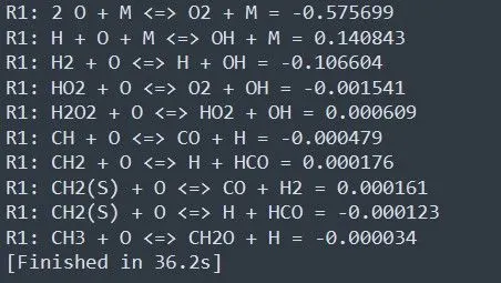
-> These are the reactions for which the sensitivity is calculated by cantera.

-> Note that the sensitivity is highest for H + O + M<=> OH +M (i.e it will take quick time to ignite vigorously).

-> The first reaction in the above figure has the least sensitivity, which means that it will take more time to ignite compared to other reactions.

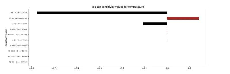
-> The above pic is a plot of sensitivity values. In the above figure, the horizontal bar graph shows sensitivity variation of reactions.

-> The right side bar shows positive temperature reactions and left side bar shows negative temperature reactions.

-> Positive temperature are faster rates than negative temperature.

-> This bar graph is very helpful to determine which reaction rate is faster and which is slower.

-> Here the reactions are showing higher and lower rates, which are very sensitive in all sensitivity reactions.

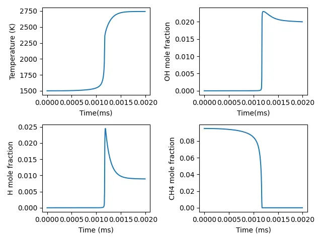
-> The above plot shows variation of molefraction of three species and temperature with time.

-> In the first plot temperature increases with time which should be the exact case.

-> In the second plot, the mole fraction of OH increases, which signifies the formation of products.

-> The trend is similar for the third plot.

-> In the fourth plot, the molefraction of CH4 decreases, because the reactants get used up to form products and hence is the variation.

Thus the sensitivity analysis is carried out using gri30.xml and the plots are shown.