Week 3 - Adiabatic Flame Temperature calculation

Adiabatic flame temperature calculation using python

In this assignment, we are going to write a code to calculate AFT(Adiabatic Flame Temperature) for a given reaction mechanism. Also, we will try to observe the variation of the AFT with varying equivalent ratios, with varying heat losses , with number if carbon atoms,etc.

Theory

Consider a combustion process that takes place adiabatically in a closed system with negligible changes in Kinetic energy and potential energy. For such a process, adiabatic flame temperature is defined as the maximum temperature that can be achieved by the products for the given reactants.

We define two adiabatic flame temperatures: one for constant-pressure combustion and one for constant-volume. If a fuel–air mixture burns adiabatically at constant pressure, the standardized enthalpy of the reactants at the initial state (say, T = 298 K, P = 1 atm) equals the standardized enthalpy of the products at the fi nal state (T = Tad , P = 1 atm),or

`h_(reac)(T_i,P)=h_(roduct)(T_(ad),P)`

The above statement expressed in terms of first law of thermodynamics is called Adiabatic flame temperature at constant pressure. Conceptually, the adiabatic fl ame temperature is simple; however, evaluating this quantity requires knowledge of the composition of the combustion products. At typical flame temperatures, the products dissociate and the mixture comprises many species.

There is also another AFT called Adiabatic Flame temperature at constant volume,which we might require in an ideal Otto-cycle analysis, for example. Again recalling that from first law of thermodynamics, we get

`U_(reac)(T_i,P_i)_=U_(pro)(T_(ad),P_f)`

which can be rewritten as `H_(reac)-H_(pro) -V(P_i-P_f)=0`

Applying ideal gas law to the above equation, we get

`H_(reac)-H_(pro) -R_u(n_(reac)T_i- n_(pro)T_(ad) )=0`

Using these two above equations, we can solve for AFT for two different cases.

Equivalence ratio`(Phi)` is defined as the ratio of fuel to air ratio for an actual case to that corresponding to a stoichiometric one i.e

`Phi=(f/a)_(actual)/(f/a)_(st)`

The general reactions involving Equivalence ratio for a lean mixture reaction is

For a fuel rich mixture, the reaction can be written as follows:

An equivalence ratio of 1 corresponds to a stoichiometric balanced mixture while a ratio of>1 corresponds to that of a fuel rich case(more fuel for given air) and with a ratio of < 1 corresponding to that of a fuel-lean case(less fuel for given air)

Programming methodology:

At first, we need to understand the programming methodology. To determine AFT of a mixture, we need to use NASA polynomials and their corresponding coefficient values so that we get accurate results of the same.

At first, a function is defined to calculate the value of the polynomial. SInce we are more concerned with the enthalpy of the fluid, we shall be using the same as shown below:

`(DeltaH)/(RT)=a_1+a_2*T_2/2 +a_3*T_3^2/3 +a4*T_4^3/4 +a5*T_5^4/5+a_6/T_6`

Next, the values of the polynomials are stored in an array.

Next, another function is defined such that we are able to calculate the enthalpy of the reaction, or the internal energy or comparing different alkanes and alkenes.

Once done, we shall be using Newton-Raphson method to calculate the adiabatic flame temperature by providing a guess value and storing these values in an array to draw suitable comparisons.

We shall also be using numpy and matplotlib modules which are predefined so as to use functions and plot graphs respectively, so that a comparative study can be carried out.

For each case, the code has been written in a modular fashion so that this case can be applied for all the cases as shown below:

1. For constant Volume process

Here, we assume that methane is contained in a constant volume chamber and we will write a program in Python to plot the effect of equivalence ratio on the final adiabatic flame temperature.

Also we will calculate the results with Cantera for varying equivalence ratios using the equilibrate method, assuming that N2 is present

For a constant volume process, we define AFT at constant volume which has the following condition:

`U_(reac)(T_i,P_i)_=U_(pro)(T_(ad),P_f)`

Here we will be implementing this into the code. Note that in this case, our species is methane and it undergoes combustion reaction in this manner as follows:

`CH_4 + 2(O_2+3.76N_2)->CO_2+2H_2O+7.52N_2`

On the left hand side, we have the reactants, which are at standard temperature(298.15K) and we will be using the second set of seven values from NASA thermodynamic data file.

On the right hand side, we habe the products, which are slated to be at higher temperature with Adiabatic temperature being the final one.

We will also be importing Cantera into our module so as to draw comparison between numerical value and the one generated by cantera.

"""
to solve For AFT for the reaction
CH4+2O2->CO2+2H2O (stoichoimetric)
CH4+2/phi(O2+3.76N2)->CO2+2H2O+(2/phi -2)O2+7.52/phiN2 	(fuel lean)
CH4+2/phi(O2+3.76N2)->(4/phi -3)CO2 + (4- /phi)CO +2H2O+7.52/phiN2	(fuel rich)
"""
import math as ma
import numpy as np
import matplotlib.pyplot as plt
def h(T,coeffs):
	#function for enthalpy calculation
	#for constant volume AFT
	R=8.314 #J/molK
	a1=coeffs[0]
	a2=coeffs[1]
	a3=coeffs[2]
	a4=coeffs[3]
	a5=coeffs[4]
	a6=coeffs[5]
	return (a1 + a2*T/2 +a3*pow(T,2)/3 +a4*pow(T,3)/4 +a5*pow(T,4)/5 +a6/T)*R*T
ch4_coeff_l=[5.14987613E+00, -1.36709788E-02, 4.91800599E-05, -4.84743026E-08, 1.66693956E-11, -1.02466476E+04, -4.64130376E+00]
o2_coeffs_l=[3.78245636E+00, -2.99673416E-03, 9.84730201E-06, -9.68129509E-09, 3.24372837E-12, -1.06394356E+03, 3.65767573E+00]
n2_coeffs_h=[0.02926640E+02, 0.14879768E-02, -0.05684760E-05, 0.10097038E-09, -0.06753351E-13, -0.09227977E+04, 0.05980528E+02]
n2_coeffs_l=[0.03298677E+02, 0.14082404E-02, -0.03963222E-04, 0.05641515E-07, -0.02444854E-10, -0.10208999E+04, 0.03950372E+02]
co2_coeffs_h=[3.85746029E+00, 4.41437026E-03, -2.21481404E-06, 5.23490188E-10, -4.72084164E-14, -4.87591660E+04, 2.27163806E+00]
h2o_coeffs_h=[3.03399249E+00, 2.17691804E-03, -1.64072518E-07, -9.70419870E-11, 1.68200992E-14, -3.00042971E+04, 4.96677010E+00]
co_coeff_h=[2.71518561E+00, 2.06252743E-03, -9.98825771E-07, 2.30053008E-10, -2.03647716E-14, -1.41518724E+04, 7.81868772E+00]
o2_coeffs_h=[3.28253784E+00, 1.48308754E-03, -7.57966669E-07, 2.09470555E-10, -2.16717794E-14, -1.08845772E+03, 5.45323129E+00]

def f(T,phi):
	T_std=298.15
	R=8.314
	h_co2_p=h(T,co2_coeffs_h)
	h_h2o_p=h(T,h2o_coeffs_h)
	h_n2_p=h(T,n2_coeffs_h)
	h_ch4_r=h(T_std,ch4_coeff_l)
	h_o2_r=h(T_std,o2_coeffs_l)
	h_n2_r=h(T_std,n2_coeffs_l)
	h_co_p=h(T,co_coeff_h)
	h_o2_p=h(T,o2_coeffs_h)
	#stoichiometry
	if phi==1:
		H_reac=h_ch4_r + 2*h_o2_r + 3.76*2*h_n2_r
		H_prod=h_co2_p + 2*h_h2o_p + 3.76*2*h_n2_p
		n_reac=1+2+7.52
		n_prod=1+2+7.52
	#rich mixture
	if phi>1:
		H_reac=h_ch4_r + (2/phi)*h_o2_r + 7.52*h_n2_r/phi
		H_prod=((4/phi) -3)*h_co2_p + (4- (4/phi))*h_co_p + 2*h_h2o_p + 7.52*h_n2_p/phi
		n_reac=1 + (2/phi) + (7.52/phi)
		n_prod=(4/phi) -3 + 4- (4/phi) +2 + (7.52/phi)
	else:
		#lean mixture
		H_reac=h_ch4_r + (2/phi)*h_o2_r + 7.52*h_n2_r/phi
		H_prod=h_co2_p + 2*h_h2o_p + ((2/phi)-2)*h_o2_p + 7.52*h_n2_p/phi
		n_reac=1 + (2/phi) + (7.52/phi)
		n_prod=1+2+(2/phi)-2 + (7.52/phi)
	return H_reac - H_prod - R*(n_reac*T_std - n_prod*T)
phi=np.linspace(0.4,1.33,20)
def fprime(T,phi):
	return (f(T+1e-6,phi)-f(T,phi))/1e-6
T_guess=1500
T_py=[]
tol=1e-3
alpha=0.3
x=0
for i in range(0,len(phi)):
	while (abs(f(T_guess,phi[i]))>tol):
		T_guess=T_guess- alpha*f(T_guess,phi[i])/fprime(T_guess,phi[i])
		x=x+1
	T_py.append(T_guess)
T_aft_py=abs(max(T_py))	#max temp obtained from newton-raphson
print('AFT obtained from newton raphson method:',T_aft_py)

#comparing data obtained from Newton-Raphson data with that of cantera
import cantera as ca
gas=ca.Solution('gri30.xml')
T_ca=[]					#temperature to be obtained from cantera
for i in range(0,len(phi)):
	"""
	CH4+2O2->CO2+2H2O (stoichoimetric)
	CH4+2/phi(O2+3.76N2)->CO2+2H2O+(2/phi -2)O2+7.52/phiN2 	(fuel lean)
	CH4+2/phi(O2+3.76N2)->(4/phi -3)CO2 + (4- /phi)CO +2H2O+7.52/phiN2	(fuel rich)
	"""
	#to obtain molefraction because phi varies
	total_moles=1+(2/phi[i]) +(7.52/phi[i])
	ch4_moles=1/total_moles
	o2_moles=(2/(phi[i]*total_moles))
	n2_moles=(7.52/(phi[i]*total_moles))
	gas.TPX=298.15,101325,{'CH4':ch4_moles,'O2':o2_moles,'N2':n2_moles}
	gas.equilibrate('UV','auto')
	T_ca.append(gas.T)

T_aft_ca=abs(max(T_ca))	
print('AFT from cantera:',T_aft_ca)		#max temperature obtained from cantera
plt.plot(phi,T_py,color='red')
plt.plot(phi,T_ca,color='green')
plt.xlabel('Equivalence ratio')
plt.ylabel('Temperature')
plt.legend(['Python','Cantera'])
plt.title('Variation of AFT with equivalence ratio')
plt.show()

AFT from newton-Raphson method:2795.9484K

AFT from cantera :2602.6366K

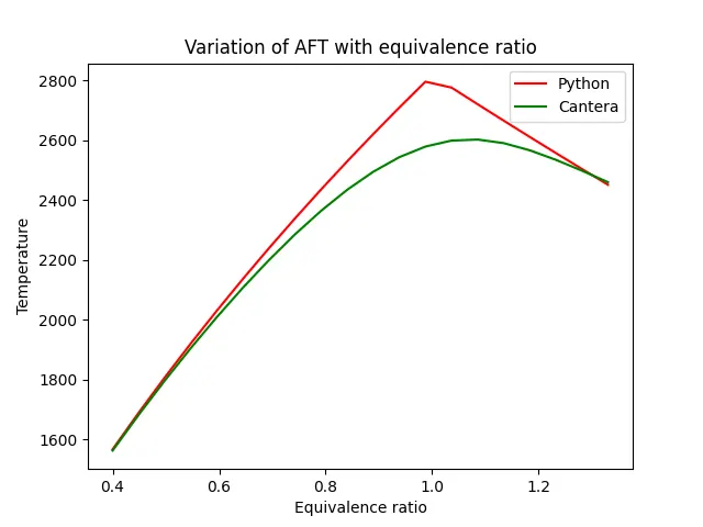
• Note that the AFT obtained from newton-Raphson method is larger than that obtained from cantera.
• This is due to the fact that in our code, we assumed only 3-4 products
• Whereas cantera calculates it for all the species and if there are a lot of products, the energy dissipated from the combustion process is going to raise the temperature of the product species and hence our value falls lower than that obtained by newton-raphson method.
• The time taken to get the results in Cantera is quicker than it takes by going with Newton-Raphson method.
• The AFT increases as the equivalence ratio increases upto a point slightly ahead of 1 i.e 1.05. It is
  interesting to note that the maximum flame temperature occurs not atstoichiometric, but, rather, at a slightly rich equivalence ratio.
• That the maximum temperature is at a slightly rich equivalence ratio is a consequence of both the heat of combustion and heat capacity of the products declining beyond `Phi=1`

2. Flame temperature variation with Heat loss (In constant pressure-chamber)

In this code, let us consider a constant pressure reactor with heat loss. The reactor is initially set at STP conditions.

The task is to vary the heat loss term by multiplying the “maximum heat loss” with a factor known as H_loss_factor. Example, H_loss_factor = 0.5 would mean a heat loss for that reaction that is equal to 50% of the maximum possible heat loss.

We shall write a code that multiplies the heat of reactants by the so-called heat loss factor

# Variation of AFT with heat loss
# H_reactant to be multiplied by numbrs from 0.1 to 1
import matplotlib.pyplot as plt
import math
import numpy as np
def h(T,coeffs):
	#function to evaluate enthalpy
	R=8.314
	a1=coeffs[0]
	a2=coeffs[1]
	a3=coeffs[2]
	a4=coeffs[3]
	a5=coeffs[4]
	a6=coeffs[5]

	return (a1 + a2*T/2 + a3*pow(T,2)/3 + a4*pow(T,3)/4 + a5*pow(T,4)/5 + a6/T)*R*T

ch4_coeffs_l=[5.14987613E+00, -1.36709788E-02, 4.91800599E-05, -4.84743026E-08, 1.66693956E-11, -1.02466476E+04, -4.64130376E+00]
o2_coeffs_l=[3.78245636E+00, -2.99673416E-03, 9.84730201E-06, -9.68129509E-09, 3.24372837E-12, -1.06394356E+03, 3.65767573E+00]
n2_coeffs_h=[0.02926640E+02, 0.14879768E-02, -0.05684760E-05, 0.10097038E-09, -0.06753351E-13, -0.09227977E+04, 0.05980528E+02]
n2_coeffs_l=[0.03298677E+02, 0.14082404E-02, -0.03963222E-04, 0.05641515E-07, -0.02444854E-10, -0.10208999E+04, 0.03950372E+02]
co2_coeffs_h=[3.85746029E+00, 4.41437026E-03, -2.21481404E-06, 5.23490188E-10, -4.72084164E-14, -4.87591660E+04, 2.27163806E+00]
h2o_coeffs_h=[3.03399249E+00, 2.17691804E-03, -1.64072518E-07, -9.70419870E-11, 1.68200992E-14, -3.00042971E+04, 4.96677010E+00]

def f(T,HL_factor):
	h_co2_p=h(T,co2_coeffs_h)
	h_n2_p=h(T,n2_coeffs_h)
	h_h2o_p=h(T,h2o_coeffs_h)
	Tstd=298.15 #std temperature
	#Lower heating value of methane
	HVL=h(Tstd,ch4_coeffs_l) + 2*h(Tstd,o2_coeffs_l) + 	7.52*h(Tstd,n2_coeffs_l) -	h(Tstd,co2_coeffs_h) -	2*h(Tstd,h2o_coeffs_h) -7.52*h(Tstd,n2_coeffs_h)
	loss=HL_factor*HVL		#HL_factor->heat loss factor to be multiplied from 0.1 to 1
	H_products=h_co2_p+ 2*h_h2o_p + 7.52*h_n2_p
	
	h_ch4_r=h(Tstd,ch4_coeffs_l)
	h_o2_r=h(Tstd,o2_coeffs_l)
	h_n2_r=h(Tstd,n2_coeffs_l)

	H_reactants=h_ch4_r + 2*h_o2_r + 7.52*h_n2_r
	return H_products - H_reactants + loss

def fprime(T,HL_factor):
	return (f(T+1e-6,HL_factor)-f(T,HL_factor))/1e-6 

T_guess=1500
tolerance=1e-3 
c=0
T_aft=[]
HL_factor=np.linspace(0.1,1,10)
alpha=0.2
for i in range(0,len(HL_factor)):
	while (abs(f(T_guess,HL_factor[i]))>tolerance):
		T_guess=T_guess - alpha*(f(T_guess,HL_factor[i])/fprime(T_guess,HL_factor[i]))
		c=c+1
	T_aft.append(T_guess)
plt.plot(HL_factor,T_aft,color='red')
plt.xlabel('Heat loss factor')
plt.ylabel('Adiabatic Flame Temperature')
plt.title('Effect of heat Loss on AFT')
plt.show()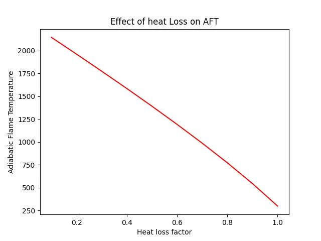

Notice that as the heat loss factor increases, the adiabatic flame temperature decreases.

It is due to the fact that less heat is available for the reactants and as a result, the species do not undergo combustion and hence we get a lot of soot(black carbon)

Thus the variation of AFT with heat loss factor is studied.

3. Adiabatic flame temperature variation with respect to Alkane, Alkene, Alkyne :

ALkanes are saturated organic compounds which have the general formula `C_nH_(2n+2)`

Alkenes are undaturated organic compounds which have the general formula `C_nH_(2n)`

Alkynes are undaturated organic compounds which have the general formula `C_nH_(2n-2)`

Note that n denotes no of carbon atoms.

The logic used in this code is based on the above analogy i.e. for a fixed number of carbon atoms(2), we study how the bond structure affects the AFT of the reaction mixture attained after combustion.

# variation of AFT with alkane,alkene,alkyne(two carbon atom molecule-ethane,ethene,ethyne)
import matplotlib.pyplot as plt
import numpy as np
def h(T,coeffs):
	#function to evaluate enthalpy
	R=8.314
	a1=coeffs[0]
	a2=coeffs[1]
	a3=coeffs[2]
	a4=coeffs[3]
	a5=coeffs[4]
	a6=coeffs[5]

	return (a1 + a2*T/2 + a3*pow(T,2)/3 + a4*pow(T,3)/4 + a5*pow(T,4)/5 + a6/T)*R*T

c2h4_coeffs_l=[3.95920148E+00, -7.57052247E-03, 5.70990292E-05, -6.91588753E-08, 2.69884373E-11, 5.08977593E+03, 4.09733096E+00]
o2_coeffs_l=[3.78245636E+00, -2.99673416E-03, 9.84730201E-06, -9.68129509E-09, 3.24372837E-12, -1.06394356E+03, 3.65767573E+00]
n2_coeffs_h=[0.02926640E+02, 0.14879768E-02, -0.05684760E-05, 0.10097038E-09, -0.06753351E-13, -0.09227977E+04, 0.05980528E+02]
n2_coeffs_l=[0.03298677E+02, 0.14082404E-02, -0.03963222E-04, 0.05641515E-07, -0.02444854E-10, -0.10208999E+04, 0.03950372E+02]
co2_coeffs_h=[3.85746029E+00, 4.41437026E-03, -2.21481404E-06, 5.23490188E-10, -4.72084164E-14, -4.87591660E+04, 2.27163806E+00]
h2o_coeffs_h=[3.03399249E+00, 2.17691804E-03, -1.64072518E-07, -9.70419870E-11, 1.68200992E-14, -3.00042971E+04, 4.96677010E+00]
c2h6_coeffs_l=[4.29142492E+00, -5.50154270E-03, 5.99438288E-05, -7.08466285E-08, 2.68685771E-11, -1.15222055E+04, 2.66682316E+00]
c2h2_coeffs_l=[8.08681094E-01, 2.33615629E-02, -3.55171815E-05, 2.80152437E-08, -8.50072974E-12, 2.64289807E+04, 1.39397051E+01]
Tstd=298.15
alka=h(Tstd,c2h6_coeffs_l)
alke=h(Tstd,c2h4_coeffs_l)
alky=h(Tstd,c2h2_coeffs_l)
alk=[alka,alke,alky]
alk=np.array(alk)
def f(T,alk):
	h_co2_p=h(T,co2_coeffs_h)
	h_n2_p=h(T,n2_coeffs_h)
	h_h2o_p=h(T,h2o_coeffs_h)
	h_o2_r=h(Tstd,o2_coeffs_l)
	h_n2_r=h(Tstd,n2_coeffs_l)
	 #std temperature
	if alk==alka:

		x=2
		y=6
		H_products=x*h_co2_p+ y*h_h2o_p/2 + 3.76*(x + 0.25*y)*h_n2_p
		H_reactants=alka + (x + 0.25*y)*h_o2_r + 3.76*(x + 0.25*y)*h_n2_r
	elif alk==alke:
		x=2
		y=4
		H_products=x*h_co2_p+ y*h_h2o_p/2 + 3.76*(x + 0.25*y)*h_n2_p
		H_reactants=alke + (x + 0.25*y)*h_o2_r + 3.76*(x + 0.25*y)*h_n2_r
	elif alk==alky:
		x=2
		y=2
		H_products=x*h_co2_p+ y*h_h2o_p/2 + 3.76*(x + 0.25*y)*h_n2_p
		H_reactants=alky + (x + 0.25*y)*h_o2_r + 3.76*(x + 0.25*y)*h_n2_r
	return H_products - H_reactants
	
def fprime(T,alk):
	return (f(T+1e-6,alk)-f(T,alk))/1e-6

"""	h_c2h2_r=h(Tstd,c2h2_coeffs_l)
	h_c2h6_r=h(Tstd,c2h6_coeffs_l)
	h_o2_r=h(Tstd,o2_coeffs_l)
	h_n2_r=h(Tstd,n2_coeffs_l)
	h_c2h4_r=h(Tstd,c2h4_coeffs_l)
"""
T_guess=1500
tol=1e-3
alpha=0.3
T_aft=[]
for i in alk:
	while abs(f(T_guess,i))>tol :
		T_guess=T_guess - alpha*(f(T_guess,i)/fprime(T_guess,i))
	T_aft.append(T_guess)
print(T_aft)
plt.figure()
plt.bar(['C2H6','C2H4','C2H2'],T_aft)
plt.ylabel('Variation of AFT')
plt.title('Variation of AFT with bonds')
plt.show()

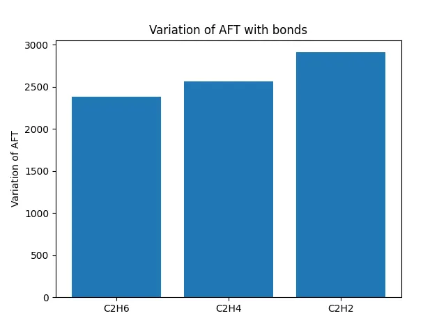
As can be seen above the AFT of the species increases for a given number of carbon atoms.

This is due to the fact that the more bonds present in the case of Alkene and alkynes possess more bonding energy and hence require more energy to split them resulting in higher Adiabatic flame temperatures as shown above.

4. Adiabatic flame temperature variation with respect to number of Carbon atom chains :

In this code,for a general alkane, we are going to plot the effect of the number of carbon atoms (from 1 to 3) on the final temperature assuming no heat loss in the combustion chamber(adiabatic case).

Loops are introduced here so as to make this code appear modular for a wide range of alkane carbon compounds.

""" to plot variation of AFT with increasing number of carbon atoms
"""
import matplotlib.pyplot as plt
import numpy as np
def h(T,coeffs):
	R=8.314
	a1=coeffs[0]
	a2=coeffs[1]
	a3=coeffs[2]
	a4=coeffs[3]
	a5=coeffs[4]
	a6=coeffs[5]	

	return (a1 + a2*T/2 + a3*pow(T,2)/3 + a4*pow(T,3)/4 + a5*pow(T,4)/5 + a6/T)*R*T

ch4_coeffs_l=[5.14987613E+00, -1.36709788E-02, 4.91800599E-05, -4.84743026E-08, 1.66693956E-11, -1.02466476E+04, -4.64130376E+00]
o2_coeffs_l=[3.78245636E+00, -2.99673416E-03, 9.84730201E-06, -9.68129509E-09, 3.24372837E-12, -1.06394356E+03, 3.65767573E+00]
n2_coeffs_h=[0.02926640E+02, 0.14879768E-02, -0.05684760E-05, 0.10097038E-09, -0.06753351E-13, -0.09227977E+04, 0.05980528E+02]
n2_coeffs_l=[0.03298677E+02, 0.14082404E-02, -0.03963222E-04, 0.05641515E-07, -0.02444854E-10, -0.10208999E+04, 0.03950372E+02]
co2_coeffs_h=[3.85746029E+00, 4.41437026E-03, -2.21481404E-06, 5.23490188E-10, -4.72084164E-14, -4.87591660E+04, 2.27163806E+00]
h2o_coeffs_h=[3.03399249E+00, 2.17691804E-03, -1.64072518E-07, -9.70419870E-11, 1.68200992E-14, -3.00042971E+04, 4.96677010E+00]
c2h6_coeffs_l=[4.29142492E+00, -5.50154270E-03, 5.99438288E-05, -7.08466285E-08, 2.68685771E-11, -1.15222055E+04, 2.66682316E+00]
c3h8_coeffs_l=[0.93355381E+00, 0.26424579E-01, 0.61059727E-05, -0.21977499E-07, 0.95149253E-11, -0.13958520E+05, 0.19201691E+02]

def f(T,no_of_carbon):		#no of carbon atoms
	"""
	Recall that since we are dealing with alkanes, its general variation is CnH(2n+2) 
	We will be using that variation
	"""
	Tstd=298.15 #std temperature
	h_co2_p=h(T,co2_coeffs_h)
	h_n2_p=h(T,n2_coeffs_h)
	h_h2o_p=h(T,h2o_coeffs_h)
	h_o2_r=h(Tstd,o2_coeffs_l)
	h_n2_r=h(Tstd,n2_coeffs_l)	
	H_products=no_of_carbon*h_co2_p+ (2*no_of_carbon + 2)*h_h2o_p/2 + (6*no_of_carbon + 2)*h_n2_p/4			
	
	if no_of_carbon==1:
		h_ch4_r=h(Tstd,ch4_coeffs_l)
		H_reactants=h_ch4_r + (6*no_of_carbon + 2)*h_o2_r/4 + (6*no_of_carbon + 2)*h_n2_r/4
	elif no_of_carbon==2:
		h_c2h6_r=h(Tstd,c2h6_coeffs_l)
		H_reactants=h_c2h6_r + (6*no_of_carbon + 2)*h_o2_r/4 + (6*no_of_carbon + 2)*h_n2_r/4
	else :
		h_c3h8_r=h(Tstd,c3h8_coeffs_l)
		H_reactants=h_c3h8_r + (6*no_of_carbon + 2)*h_o2_r/4 + (6*no_of_carbon + 2)*h_n2_r/4
	return (H_products - H_reactants)

def fprime(T,no_of_carbon):
	return (f(T+1e-6,no_of_carbon)-f(T,no_of_carbon))/1e-6

T_guess=1500
T_aft=[]
no_of_carbon=[1,2,3]
tolerance=1e-3
alpha=0.3
for c in no_of_carbon:
	while (abs(f(T_guess,c))>tolerance):
		T_guess=T_guess - alpha*(f(T_guess,c)/fprime(T_guess,c))
	T_aft.append(T_guess)
print(T_aft)
plt.plot(no_of_carbon,T_aft,'-o',color='red')
plt.xlabel('No of carbon bonds')
plt.ylabel('AFT')
plt.title('Variation of Adiabatic with no of carbon atoms')
plt.show()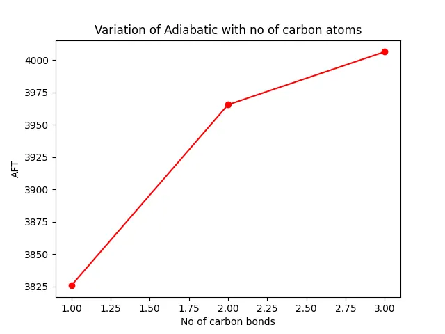

Species	AFT
Methane	3825.650198197418
Ethane	3965.531820903354
Propane	4006.4538330662635

As can be seen above, the AFT shows a drastic variation with respect to the number of carbon atoms as shown.

This is due to the fact that more number of carbon atoms are broken down which requires more energy to be supplied which inturn rises the temperature in the combustion chamber.

Thus the AFT flame calculation is carried out for different cases and the results are observed.