Week 1- Mixing Tee

MIXING TEE JOINT FLOW SIMULATION IN ANSYS FLUENT

In this challenge, a mixing tee is simulated with two different cases-a longer pipe and a shorter pipe. A CFD analysis is carried out over the mixing tee subjected to two cases which are enlisted below:

Case 1:

Short mixing tee with a hot inlet velocity of 3 m/s and with momentum ratio of 2 and 4(momentum ratio=(velocity at cold entry)/(velocity at hot entry)

Case 2:

Long mixing tee with a hot inlet velocity of 3 m/s and with momentum ratio of 2 and 4(momentum ratio=(velocity at cold entry)/(velocity at hot entry))

The end result of this challenge will be to perform the following:

• Compare cell values from two cases above and compare the temperature at the outlet.
• Compare velocity and temperature contour plots on the cut planes along and across the pipe for two cases.
• Compare velocity and temperature line plots along and across the length of the pipe.
• Perform Mesh independent study for any one case.
• To discuss the effect of length and momentum ratio on results.

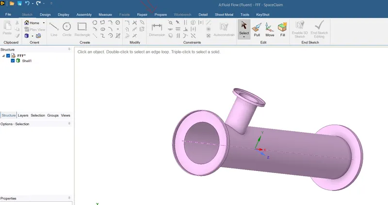
A mixing tee, as shown above is used in appliances involving mixing of fluids at different temperatures. It consists of a short pipe through which cold fluid enters at comparatively higher speeds than the hot air that enters through the long tube. The fluids can be of same physical properties but are of different chemical properties. Applications where pipeline mixing with tees is used include low viscosity mixing such as waste water treatment, air conditioners, blending of oils and petrochemical products. The main interest in this challenge is to understand the process happening in the mixing of flows by using GUI power of Ansys FLUENT and plotting contours of temoerature variation and velocity variation.

To analyse a problem via CFD technique, it involves three steps:

->Pre Processing

->Solving

->Post-Processing

Preprocessing: This process involves prepping up the geometry model for the required simulation. Here the geometry is imported, fluid volume is extracted and some other steps are followed. Following that, the model is meshed appropriately.

Solving:This process involves applying relevant initial conditions,boundary conditions,turbulent models,etc.

PostProcessing:This process is used to analyse the results obtained in the solution and allows the visualisation of the results in a more understandable manner.

PROCEDURE

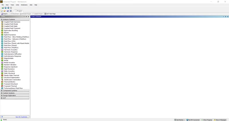
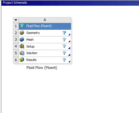
The procedure involves first setting up the project site by drag and drop of fluent icon into the project schematic window, as shown below

In the next step, the cad file is to be imported from the directory to the geometry menu, where we use spaceclaim to clean up the geometry as shown below.

The imported geometry looks like this in spaceclaim. To remove the edges and to make sure that only the volume that the fluid moves through remains, click on prepare menu and click on Volume extract option as shown below.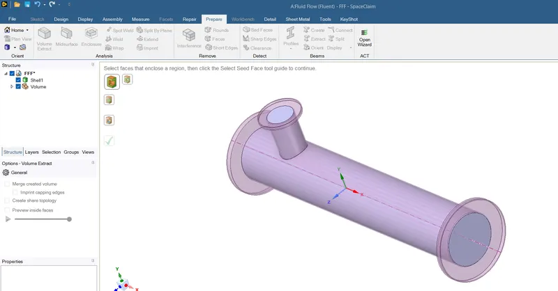

Click on shell1 from the structure tree and right click on it and select 'suppress for physics' option. This will make sure that only the blue coloured element remains intact for analysis. Close the spaceclaim.

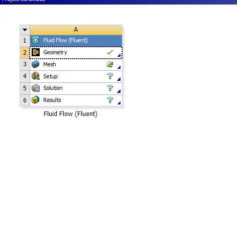
The tree gets updated like this. Double clcik on mesh,and it will open a window.

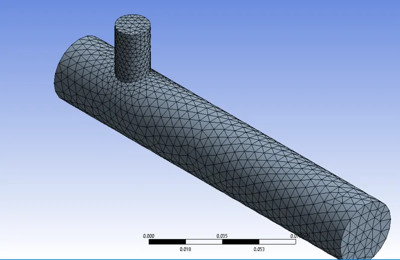
Once the meshing is done, the next step is to provide initial values and boundary conditions to the solver by specifying it in setup menu. Double click on it.

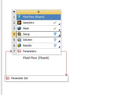
Since there is mixing of fluids of different temperatures,click on energy equation. Next specify the boundary conditions in the menu as given in the challenge and run the solution for 200 iterations and repeat the steps for different cases.

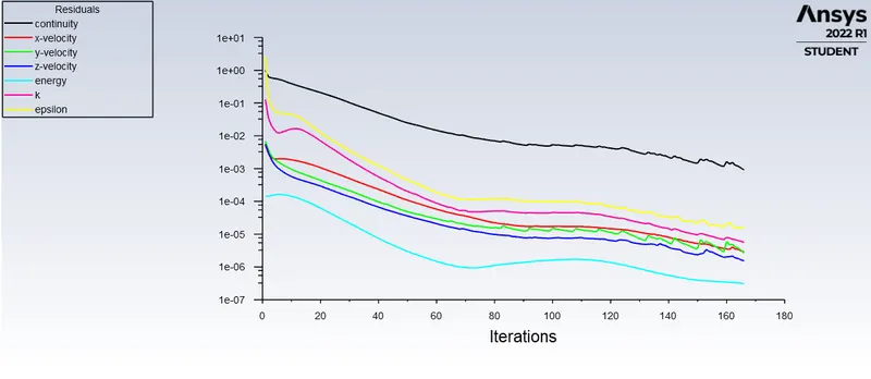
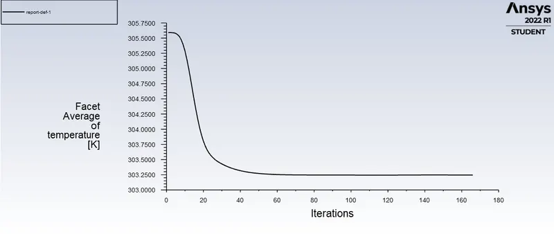
Convergence plots

Postprocessing

In this step, the results that are obtained are visualised and processed to draw meaningful inferences from it. We plot the variation of temperature and velocity across a cross-section of the pipe and along the length of the pipe.

The same procedure is repeated for all cases and subcases.

RESULTS AND DISCUSSIONS

1. Short tee with momentum ratio of 2

The results are shown below.

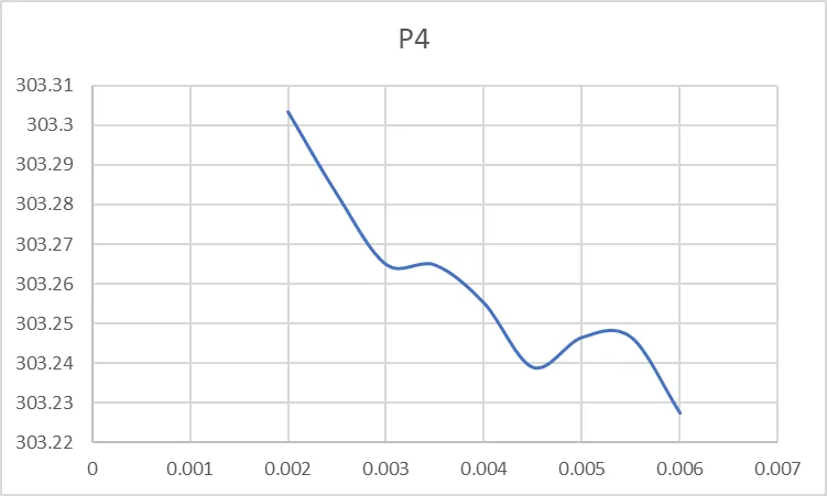
Grid independence study plotting variation of temperature as sizing of nodes increases

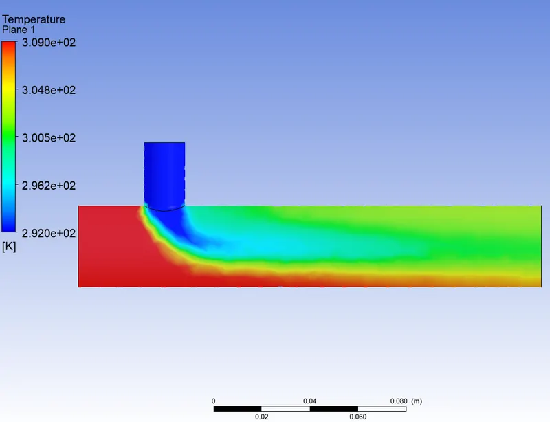
Temperature contours along the length of the pipe

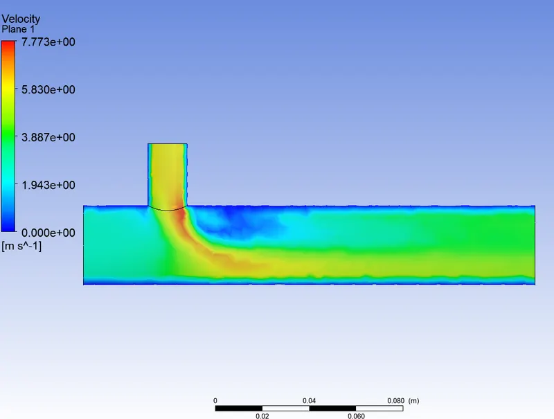
Velocity contour along the length of the pipe

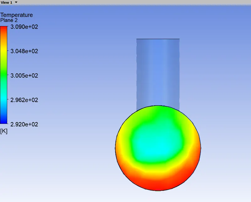
Temperature contours across a section of the tee

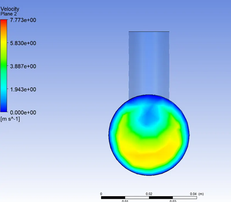
Velocity contours across a section of the tee

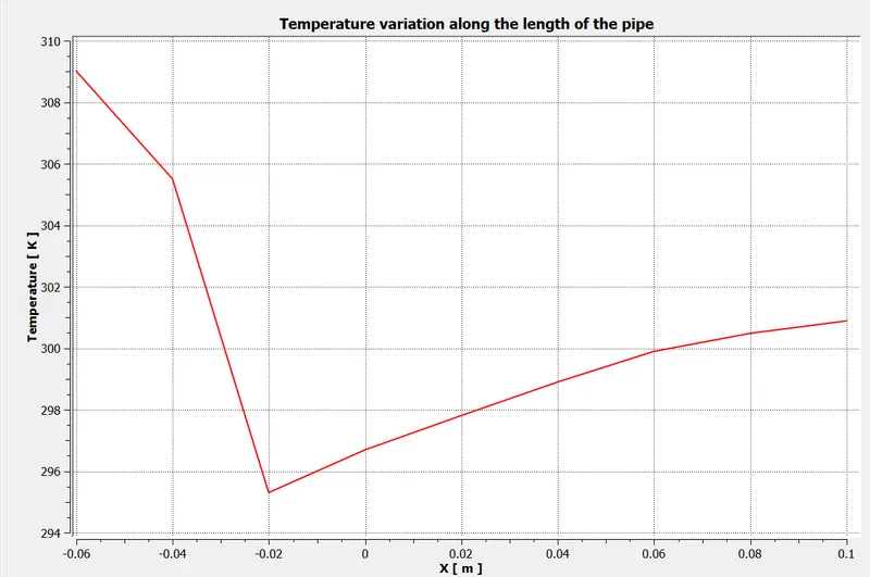
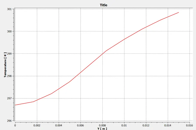
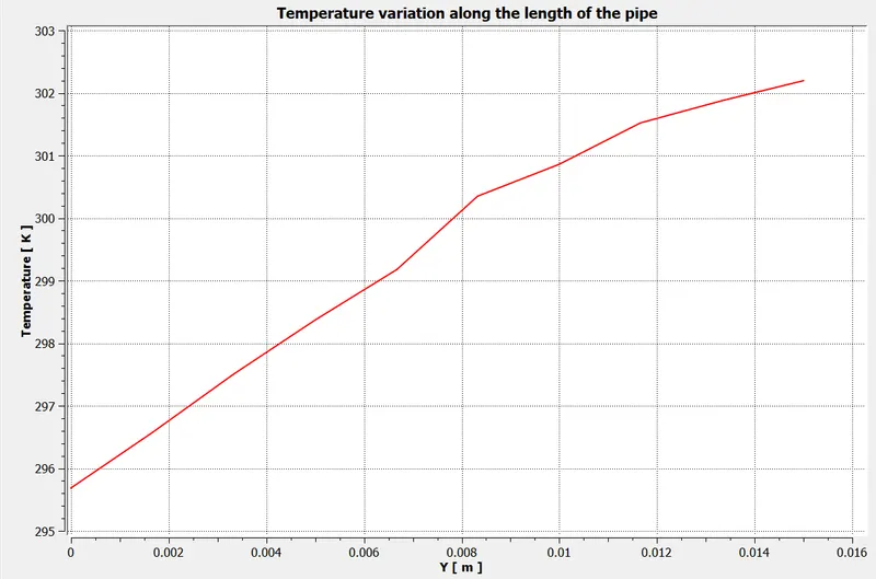
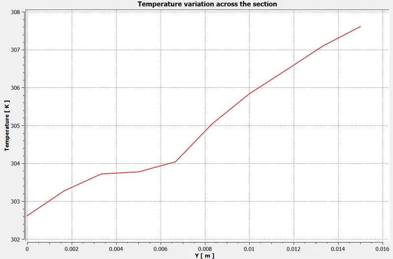
Temperature variation along the radial direction

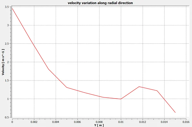
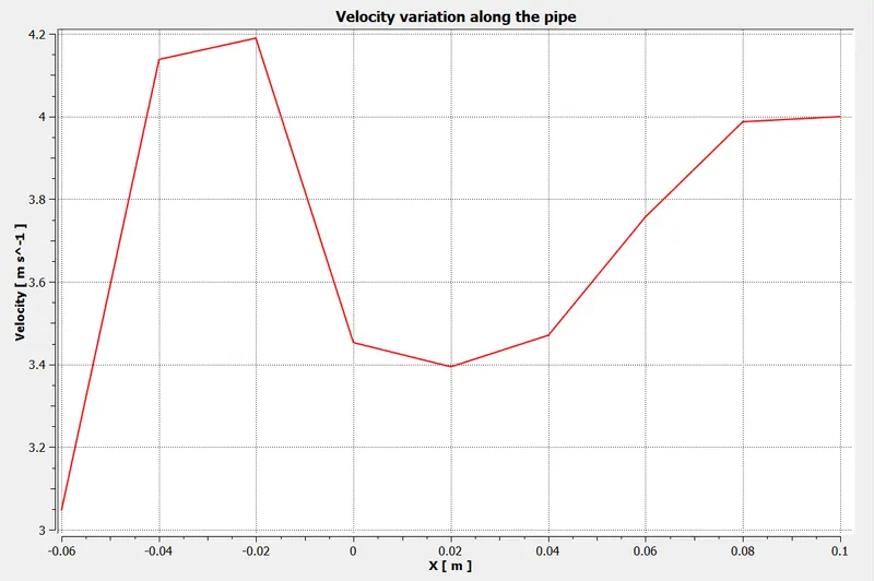
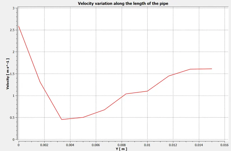
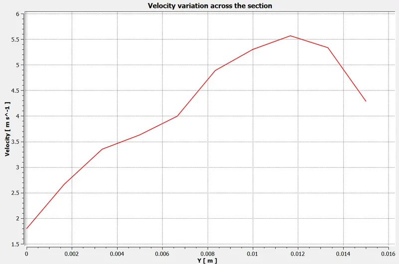
Velocity variation along the radial direction

2. Short tee with momentum ratio 4

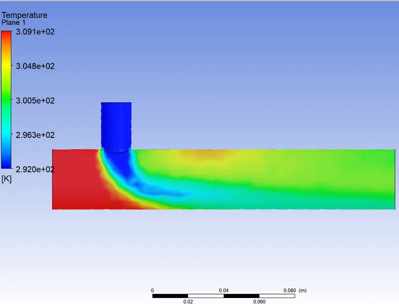
Temperature contour along the length of the pipe

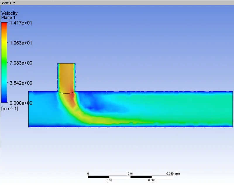
Velocity contour along the length of the pipe

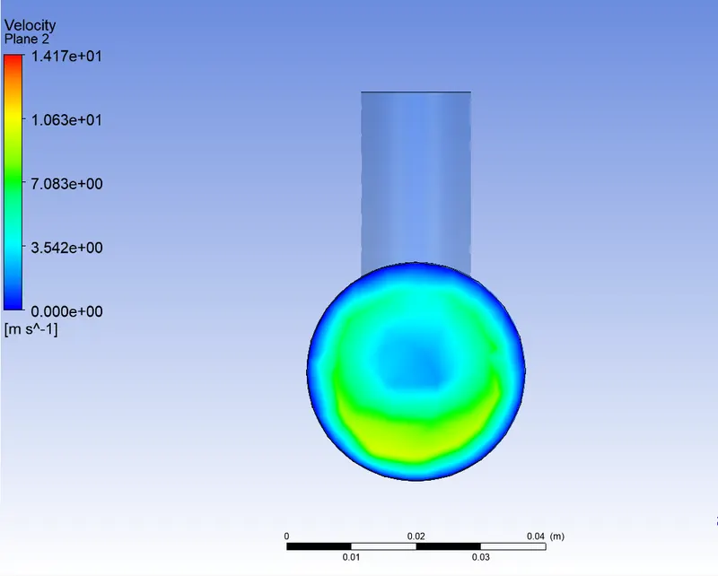
Velocity contour across the pipe diameter

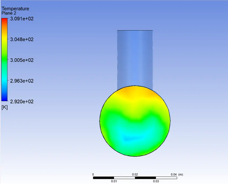
Temperature contour across the pipe diameter

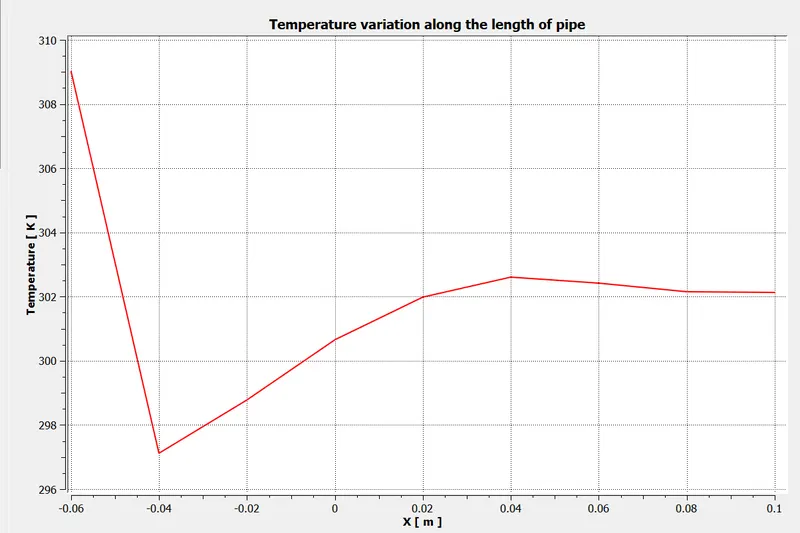
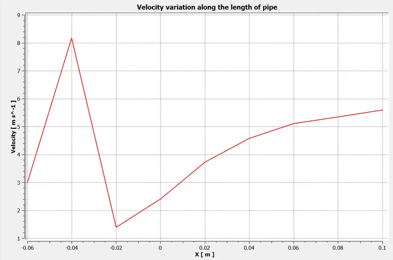
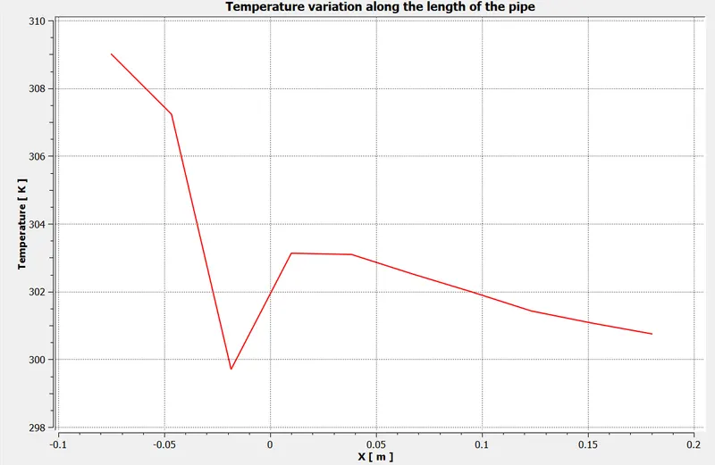
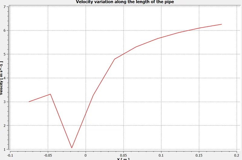
As is evident from the graphs and contours shown above, we observe that the the velocity experiences a sudden rise in its value along the length because of mixing of different speed flows with a drop in temperature. Comparing the plots for different values of momentum ratios, we see that the temperature drops and velocity increase are more abrupt with increasing momentum ratios.

3. Long tee with momentum ratio 2

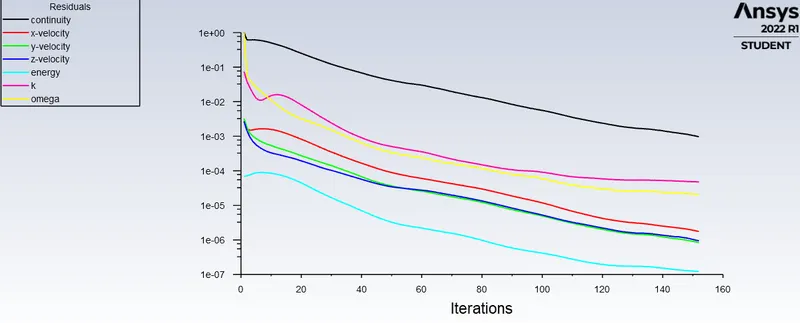
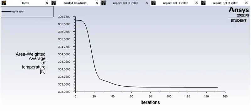
Convergence plots

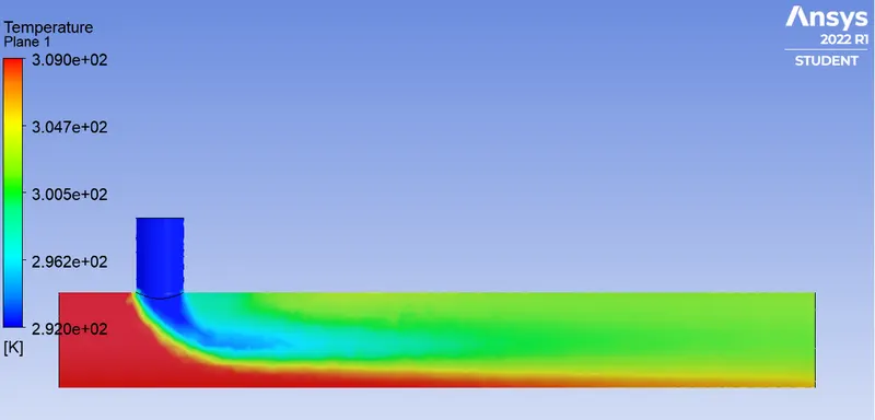
Temperature contour along the length of the pipe

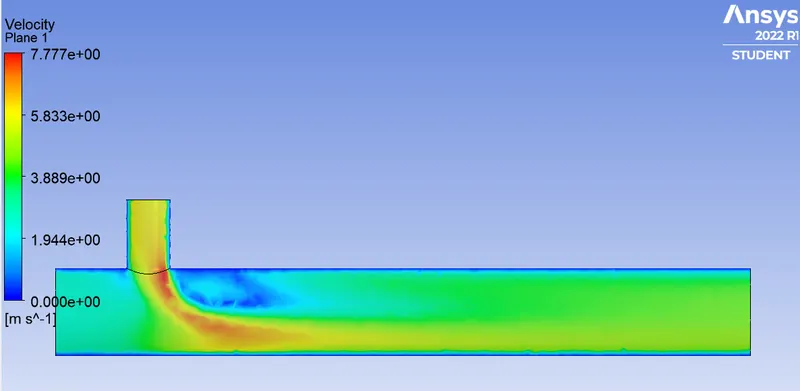
Velocity contour along the length of the pipe

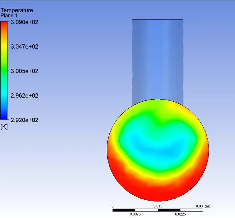
Temperature contour across the pipe

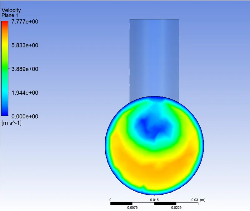
Velocity contour across the pipe

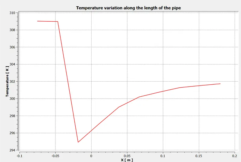
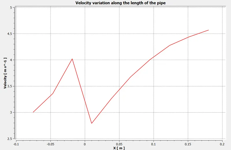
4. Long tee with momentum ratio 4

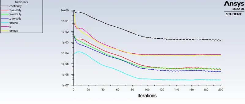
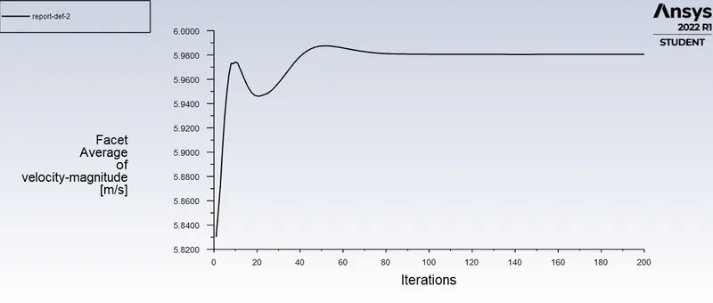
Convergence plots

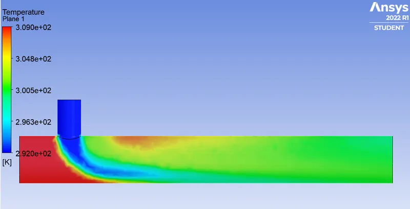
Temperature contour along the length of the pipe

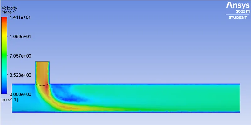
Velocity contour along the length of the pipe

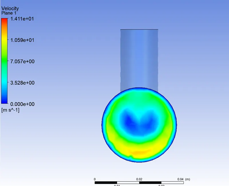
Velocity contour across the pipe

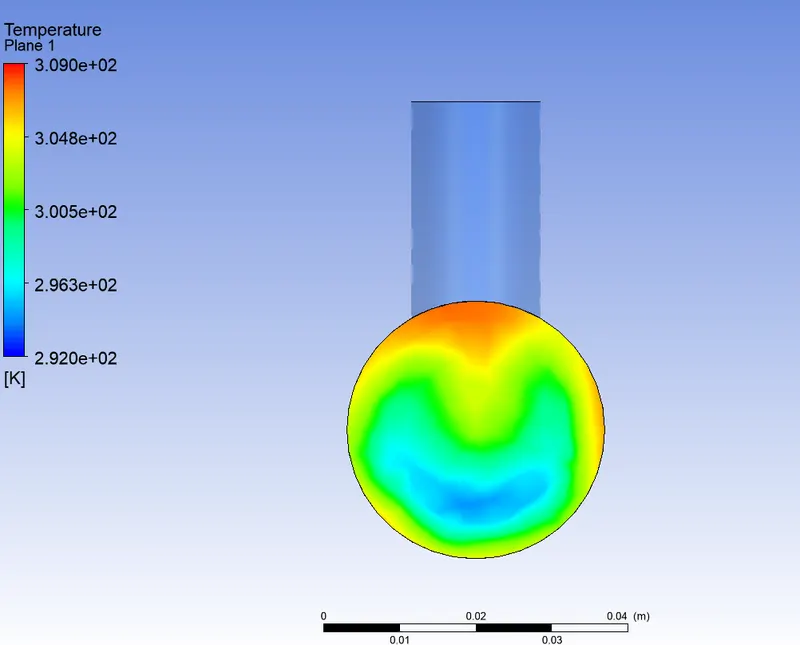
Temperature contour across the pipe

Comparison of all values

Type of tee	momentum ratio	no of iterations to converge	Avg.temperature at the outlet(in K)	Avg. Velocity at the outlet (in m/s)
Short tee	2	166	303.2274	4.4973
	4	149	300.539	6.0199
Long tee	2	323	303.323	4.477
	4	200	300.522	5.9801

The visocus model chosen was k-SST omega because it follows second order upwind scheme, which causes the solution to converge quickly for short tee. From the above values, we see that with increase in momentum ratio, the outlet velocity and the outlet temperature increases an decreases respectively. As the length of the pipe increases, the variation in temperature is less than (0.03%), which shows that length is irrelevant in this case. The grid independence study has been conducted and the results are updated above. Comparing the temperature contours, we can observe that as the momentum ratio increases, the flow diffuses more. As the length of the pipe increases for a given momentum ratio, we see that it has little to no effect in the variation of temperature and velocity.