Week 6 Challenge-FVM Fundamentals 101

FVM Fundamentals 101

Derivation

In this challenge, we shall look at the derivation of second order accurate first order scheme, followed by applying FVM formulation to the equation and describing about TVD schemes in detail.

The taylor series expansion of `f_(i+1)` about the point i is given b`

`f_(i+1)=f_i + f'_iDeltax + f''_i(Deltax^2)/(2!) + f'''_i(Deltax^3)/(3!)`

Similarly, for `f_(i-1)` about the point i is given by

`f_(i-1)=f_i - f'_iDeltax + f''_i(Deltax^2)/(2!) - f'''_i(Deltax^3)/(3!)`

Subtracting the above equations, we get

`f_(i+1) - f_(i-1)=2f'_iDeltax + O(Deltax^3)`

Dividing dy `2Deltax` on both sides, we get

`(f_(i+1) - f_(i-1))/(2Deltax)=f'_i + O(Deltax^2)`

Thus we get a first order dervative which is second order accurate.

FVM FORMULATION

The differential equation is `(partial(rhophi))/(partialt) + nabla.(rhoUphi)=0`

Gauss divergence theorem is a useful formulation to convert a volume integral to a surface integral and vice-versa.

The theorem states that `int_SvecA.vec(dS) = int_Vnabla.vecAdV`, where A is any property.

Applying Gauss divergence theorem to the above equation, we get

`int(partial(rhophi))/(partialt) + intnabla.(rhoUphi)=0`

Multiply by dV, we get

`int(partial(rhophi))/(partialt)dV + intnabla.(rhoUphi)dV=0`

The above equation can be rewritten by applying Gauss Divergence theorem as

`partial/(partialt)int_VrhophidV + int_Srhophivec(U).vec(dS)=0`

The time derivative term can be left unchanged but the second term can be modified as

`int_Srhophivec(U).vec(dS)=sum_fvecS_f *(rhovecUphi)_f`

We have approximated the volume integral into surface integral and into a sum series which can be performed.

The continuity equation can be written as

`partial/(partialt)int_VrhophidV + sum_fvecS_f *(rhovecUphi)_f=0`

TVD schemes

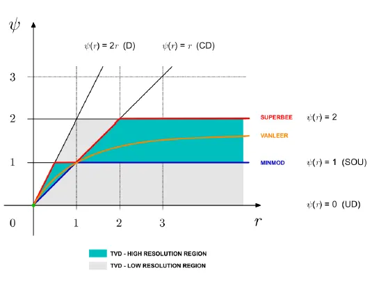
A TVD scheme, is a scheme that does not create new local undershoots and/or overshoots in the solution or amplify existing extremes. In CFD we want stable, non-oscillatory, bounded, high order schemes. The Sweby diagram (Sweby, 1984), gives the necessary and sufficient conditions for a scheme to be TVD. In the figure, the shaded area represents the admissible TVD region. However, not all limiter functions are second order.High-resolution schemes falls in the blue area and low-resolution schemes falls in the grey area. The drawback of the limiters is that they reduce the accuracy of the scheme locally to first order (low resolution scheme), when r < 0 (sharp gradient, opposite slopes or zero gradient). However, this is justified when it serves to suppress oscillations.No particular limiter has been found to work well for all problems, and a particular choice is usually made on a trial-and-error basis.

TVD is a property used in the discretisation of equations governing time-dependent gas dynamics problems. More recently, schemes with this property have also become popular in general purpose CFD solvers. The basic upwind differencing scheme is the most stable and unconditionally bound scheme, but it introduces a high level of false diffusion due to its low order of accuracy. Higher order schemes, such as central differencing and QUICK can give spurious oscillations or wiggles when the Peclet number is high. When such higher order schemes are used to solve for turbulent quantities, wiggles can give physically unrealistic negative values and instability. TVD schemes are designed to address this undesirable oscillations of higher order schemes. In TVD, the tendency towards oscillation is counteracted by adding an artificial diffusion fragment or by adding a weighting towards upstream contribution.

Limited linear schemes

The limited linear scheme — as the name suggests — maintains the linear scheme as much as possible to be TVD, before limiting to upwind to improve boundedness. Limited linear is a robust scheme that exhibits low diffusion, but has a disadvantage that it is not symmetric.

van Leer

This is a notable TVD schemes that exhibit low diffusion, maintain symmetry through some downwind interpolation,and have limiter functions which are continuous in gradient which avoids problems due to sudden changes in limiter values.

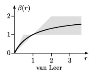
The van Leer scheme is the original limited advection scheme described by the limiter function

`beta=frac(r + |r|)(1 + |r|)`

Since `beta->2`as `r->infty`,the van Leer scheme uses relatively strong downwind interpolation.