Week 7 - Simulation of a 1D Super-sonic nozzle flow simulation using Macormack Method
AIM
To derive the conservative and non-conservative forms of the governing equations and to simulate the isentropic flow through a convergent-divergent nozzle by writing a code and plotting sufficient graphs.
THEORY
SETUP
There are three steps needed to be followed here
-> The governing equations will be couched in terms of partial differential equations suitable for the time-marching solution of quasi-one-dimensional flow
->The finite-difference expressions about Macormack's technique as applied to this problem will be set-up
->The boundary conditions, timesteps etc are all specified next.
A nozzle is a device that accelerates a given mass flow of air to higher speeds by compensating the static pressure. We know that to propel a device, gases must be sent out through the nozzle. A convergent nozzle can only accelerate the flow to sonic conditions, whereas a divergent nozzle along with the convergent nozzle will help in achieving supersonic conditions.
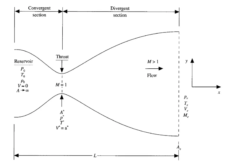
By varying the pressure ratio across the nozzle, one can obtain sufficient speeds at the exit until a limit called a Choking point beyond which any sufficient variation in the pressure won't affect the mass flow rate through the nozzle.
We know that the governing equations of mass, momentum and energy respectively are:
`del/(delt)intintintrho*dV+ intintrhoV.dS =0`
`del/(delt)intintintrho*u*dV+ intintrhouV.dS =-intintpdS` (without any body force)
`del/(delt)intintintrho(e+(V^2/2))dV+ intintrho(e+(V^2/2))V.dS =-intintpV.dS`
We have to manipulate the above equation to get the conservative and non-conservative forms of the governing equations.
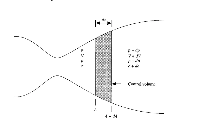
Consider a cross-section of a nozzle as shown above. Let the flowfield variables be p,v,` rho`,e where they represent pressure, velocity, density, and internal energy respectively.
Applying continuity equation to the above control volume,we get
`intintrhoV.dS=d(rhoAV)`
`implies (del(rhoA))/(delt) +(del(rhoAv))/(delx) =0`
The above is the partial differential equation for continuity equation in conservative form.
The non-conservative form can be derived from conservative form as follows:
`implies (del(rhoA))/(delt) +v(del(rhoA))/(delx) =-rhoA(delv)/(delx)`
The momentum equation
`intintrhouV.dS=-rhoV^2A+(rho+delrho)(v+delv)^2(A+delA)`
For the calculation of the pressure term,consider x component
`intintpdS=-pA+(p+dp)(A+dA)-pdA`
Substituting in the momentum equation and simplifying, we get
`(del(rhovA))/(delt)+(del(rhov^2A))/(delx)=-A*(delp)/(delx)`
This is the conservative form of the momentum equation. Let us obtain the non-conservative form of the momentum equation.
`implies (vdel(rhoA))/(delt) +(vdel(rhoAv))/(delx) =0`
Substitute the above equation in the conservative form and simplifying, we get the nonconservative form of the momentum equation as follows:
`rho(delv)/(delt)+rhov(delv)/(delx)=-(delp)/(delx)`
The Energy Equation
`(del(rho(e+v^2/2)Adx))/(delt)-rho(e+v^2/2)Av+(rho+drho)(e+de+(v+dv)^2/2)(A+dA)(v+dv)=-[-pvA+(p+dp)(v+dv)(A+dA)-pvdA]`
Simplifying the above equation,we get the conservative form of the energy equation
`(del(rho(e+v^2/2)A))/(delt) +(del(rho(e+v^2/2)Av))/(delx)=-(del(pAv))/(delx)`
The non conservative equation can be derived from conservative form as follows:
`rho(dele)/(delt)+rhov(dele)/(delx)=-p(delV)/(delx)-pv(del(lnA))/(delx)`
We know that the equation of state is `p=rho*R*T` and the heat equation is `e=underset(v)(C)*T`
Hence, we have 5 equations and 5 unknowns to solve for the nozzle flow.
At this stage, we can proceed with the above equations to set up our numerical solution. Note that the variables are expressed in dimensional form. For nozzle flows, the flow field parameters are expressed in terms of ratios like `underset(o)(P)/P` and hence we will stick to using the non-dimensional form.
Hence our new temperature will be equal to T`=`T/underset(o)(T)`
`rho'=rho/underset(o)(rho)`
`x'=x/L`
Defining the speed of the sound as `underset(o)(a)=sqrt(gamma*R*T)`
The dimensionless velocity can be written as `V'=V/underset(o)(a)`
The dimensionless time is also written as `t'=t/{L/underset(o)(a)}`
Finally we write the local area ratio to the sonic throat area in dimensionless form as `A'=A/A^**`
Returning to the above equations and writing the equations in dimensionless form,
CONTINUITY EQUATION IN NON-DIMENSIONAL FORM
`(delrho')/(delt') =-v'(delrho')/(delx') -rho'(delv')/(delx')-rho'v'(dellnA')/(delx')`
MOMENTUM EQUATION IN NON DIMENSIONAL FORM
`(delv')/(delt')=-v'(delv')/(delx')-(1/gamma)((delT')/(delx')+((T')/(rho').(delrho')/(delx')))`
ENERGY EQUATION IN NON-CONSERVATIVE FORM
`(delT')/(delt')=-v'(delT')/(delx')-(gamma-1)T'((delv')/(delx')+v'(dellnA')/(delx'))`
The above three equations in non-dimensional form are most appropriate for the time marching setup of the solution.
->FINITE DIFFERENCE EQUATIONS
To implement a finite difference solution, we divide the x-axis along with the nozzle into several discrete grid points. The points are evenly distributed along the x-axis, with `Deltax`denoting the spacing between grid points. The first point is denoted as 1, whilst the last point is denoted as N. Point i is an arbitrary grid point, with points i-1 and i+1 as the adjacent grid points. The equations are solved with MacCormack's method which is a predictor-corrector method. In the time-marching approach, remember that we know the flow-field values at time t, and we use the difference equations to solve explicitly for the variables at a time `t+Deltat`.
MacCormack's method involves a forward differencing prediction followed by backward differencing correction to eliminate the need for any second-order derivative. This method is second-order accurate.
Continuity equation can be discretized in forward scheme as follows :
`underset(i)((delrho)/(delt))^t=-underset(i)(rho^t)*(underset(i+1)(V^t)-underset(i)(V^t))/(Deltax)-underset(i)(rho^t)underset(i)(V^t)*((underset(i+1)(lnA^t)-underset(i)(lnA^t))/(Deltax))-underset(i)(V^t)*(underset(i+1)(rho^t)-underset(i)(rho^t))/(Deltax)`
The momentum equation can be discretized in forward scheme as follows:
`underset(i)((delV)/(delt))^t=-underset(i)(V^t)*(underset(i+1)(V^t)-underset(i)(V^t))/(Deltax)-(1/gamma)((underset(i+1)(T^t)-underset(i)(T^t))/(Deltax)+((underset(i)(T^t))/(underset(i)(rho^t)))(underset(i+1)(rho^t)-underset(i)(rho^t))/(Deltax) )`
The energy equation can be discretized in forward scheme as follows:
`underset(i)((delT)/(delt))^t=-underset(i)(V^t)*(underset(i+1)(T^t)-underset(i)(T^t))/(Deltax)-(gamma-1)*underset(i)(T^t)((underset(i+1)(V^t)-underset(i)(V^t))/(Deltax)+(underset(i)(V^t)(underset(i+1)(lnA^t)-underset(i)(lnA^t))/(Deltax) ))`
Once the values are computed, we obtain predicted values of `rho,V,T` denoted as follows:
`underset(i)(rho^(t+Deltat))=underset(i)(rho^(t))+underset(i)((delrho)/(delt))^t*Deltat` ---1
`underset(i)(V^(t+Deltat))=underset(i)(V^(t))+underset(i)((delV)/(delt))^t*Deltat` ---2
`underset(i)(T^(t+Deltat))=underset(i)(T^(t))+underset(i)((delT)/(delt))^t*Deltat` ---3
Moving to the corrector step, we return to the discretized form with backward differencing scheme as follows:
Continuity equation can be discretized in backward scheme as follows :
`underset(i)((delrho)/(delt))^t=-underset(i)(rho^t)*(underset(i)(V^t)-underset(i-1)(V^t))/(Deltax)-underset(i)(rho^t)underset(i)(V^t)*((underset(i)(lnA^t)-underset(i-1)(lnA^t))/(Deltax))-underset(i)(V^t)*(underset(i)(rho^t)-underset(i-1)(rho^t))/(Deltax)`
The momentum equation can be discretized in backward scheme as follows:
`underset(i)((delV)/(delt))^t=-underset(i)(V^t)*(underset(i)(V^t)-underset(i-1)(V^t))/(Deltax)-(1/gamma)((underset(i)(T^t)-underset(i-1)(T^t))/(Deltax)+((underset(i)(T^t))/(underset(i)(rho^t)))(underset(i)(rho^t)-underset(i-1)(rho^t))/(Deltax) )`
The energy equation can be discretized in backward scheme as follows:
`underset(i)((delT)/(delt))^t=-underset(i)(V^t)*(underset(i)(T^t)-underset(i-1)(T^t))/(Deltax)-(gamma-1)*underset(i)(T^t)((underset(i)(V^t)-underset(i-1)(V^t))/(Deltax)+(underset(i)(V^t)(underset(i)(lnA^t)-underset(i-1)(lnA^t))/(Deltax) ))`
Once the values are computed, we need to take the average derivative of the predictor and corrector values:
Once the values are computed, we obtain the flow-field values of `rho,V,T` denoted as follows:
`underset(i)(rho^(t+Deltat))=underset(i)(rho^(t))+underset(i)((delrho)/(delt))^t*Deltat`
`underset(i)(V^(t+Deltat))=underset(i)(V^(t))+underset(i)((delV)/(delt))^t*Deltat`
`underset(i)(T^(t+Deltat))=underset(i)(T^(t))+underset(i)((delT)/(delt))^t*Deltat`
CALCULATION OF TIMESTEP
The final step is to calculate the timestep and apply boundary conditions.
The timestep is calculated by using the below formulae:
`Deltat=C*(Deltax)/(a+V)`
For each value of V, a time step is computed at each node and the minimum value of the timestep is used.
It is reasonable to assume the boundary condition as V(1)=2V(2)-V(3);
`underset(1)(rho)=1;underset(1)(T)=1`
Since the flow is supersonic at the nozzle exit, `underset(n)(V)=2*underset(n-1)(V)-underset(n-2)(V)`
`underset(n)(rho)=2*underset(n-1)(rho)-underset(n-2)(rho)`
`underset(n)(T)=2*underset(n-1)(T)-underset(n-2)(T)`
NOZZLE SHAPE AND INITIAL CONDITION
The nozzle is assumed to vary along x-axis alone i.e A=A(x)
`A=1+2.2(x-1.5)^2 0<=x<=3`
`rho=(1-0.3146*x)`
`T=(1-0.2314*x)`
`V=(0.1+1.09x)T^.5`
With all values being declared, a program is written in MatLab employing both conservative and non-conservative forms.
MAIN CODE
n=31;
x=linspace(0,3,n);
dx=x(2)-x(1);
n_t=1400;                          %number of timesteps
C=0.5;                            %assume courant number as 0.5
Gamma=1.4;

tic
[v,mach_numb,p,rho,temp,temp_throat,rho_throat,vel_throat,machno_throat,pres_throat,mass_flow_rate]= nozzle_flow_non_conservative(n,C,dx,n_t,x,Gamma);
time_noncons=toc;

tic
[v_cons,mach_numb_cons,p_cons,rho_cons,temp_cons,temp_throat_cons,rho_throat_cons,vel_throat_cons,machno_throat_cons,pres_throat_cons,a,mass_flow_rate_cons]=nozzle_flow_conservative(n,C,dx,n_t,x,Gamma);
time_cons=toc;

%for non conservative
figure(1)
subplot(3,1,1)
axis([0 3 0 6]);
plot(x,a,'r');
xlabel('non-dimensional-length');
ylabel('Area ratio');
subplot(3,1,2)
axis([0 3 0 1]);
plot(x,p,'b');
xlabel('non-dimensional-length');
ylabel('P/{Po}');
subplot(3,1,3)
axis([0 3 0 1]);
plot(x,rho,'g');
xlabel('non-dimensional-length');
ylabel('\rho/{\rho0}');
figure(2)
subplot(3,1,1)
axis([0 3 0 4]);
plot(x,mach_numb,'c');
xlabel('non-dimensional-length');
ylabel('Mach number');
subplot(3,1,2)
axis([0 n_t 0 2]);
plot(1:n_t,temp_throat,'b');
xlabel('No of timesteps');
ylabel('Temp ratio at throat');
subplot(3,1,3)
axis([0 n_t 0 2]);
plot(1:n_t,rho_throat,'g');
xlabel('no of timesteps');
ylabel('density ratio at throat');
figure(3)
subplot(2,1,1)
plot(1:n_t,machno_throat,'c');
xlabel('no of timesteps');
ylabel('mach no at throat');
subplot(2,1,2)
plot(1:n_t,pres_throat,'r');
xlabel('no of timesteps');
ylabel('pressure ratio at throat');

%for conservative part
figure(4)
subplot(3,1,1)
axis([0 3 0 5]);
plot(x,mach_numb_cons,'r');
xlabel('Non-dimensional Length');
ylabel('Mach number');
subplot(3,1,2)
axis([0 3 0 6]);
plot(x,a,'r');
xlabel('non-dimensional-length');
ylabel('Area ratio');
subplot(3,1,3)
axis([0 3 0 1]);
plot(x,p_cons,'b');
xlabel('non-dimensional-length');
ylabel('P/{Po}');
figure(5)
subplot(3,1,1)
axis([0 3 0 2]);
plot(x,temp_cons,'g');
xlabel('non-dimensional-length');
ylabel('T/{To}');
subplot(3,1,2)
axis([0 3 0 2]);
plot(x,rho_cons,'c');
xlabel('non-dimensional-length');
ylabel('\rho/{\rhoo}');
subplot(3,1,3)
axis([0 n_t 0 1]);
plot(1:n_t,temp_throat_cons,'linewidth',2);
xlabel('No of timesteps');
ylabel('temp at the throat');
figure(6)
subplot(2,1,1)
plot(1:n_t,machno_throat_cons,'c');
xlabel('no of timesteps');
ylabel('mach no at throat');
subplot(2,1,2)
plot(1:n_t,pres_throat_cons,'r');
xlabel('no of timesteps');
ylabel('pressure ratio at throat');

%comparison of normalized mass flow rates
figure(9)
plot(x,mass_flow_rate,'c','linewidth',2);
hold on
plot(x,mass_flow_rate_cons,'g','linewidth',2);
xlabel('Non-dimensional length');
ylabel('Non dimensional massflow rate');
legend('non-conservative-form','conservative form');
Function for Conservative Form
function [v_cons,mach_numb_cons,p_cons,rho_cons,temp_cons,temp_throat_cons,rho_throat_cons,vel_throat_cons,machno_throat_cons,pres_throat_cons,a,mass_flow_rate_cons]=nozzle_flow_conservative(n,C,dx,n_t,x,Gamma)
for i=1:length(x)
    if x(i)>=0 & x(i)<=0.5
        rho_cons(i)=1;
        temp_cons(i)=1;
    end
    if x(i)>0.5 & x(i)<=1.5
        rho_cons(i)=1-0.366*(x(i)-0.5);
        temp_cons(i)=1-0.167*(x(i)-0.5);
    end
    if  x(i)>1.5 & x(i)<=3.0
        rho_cons(i)=0.634-0.3879*(x(i)-1.5);
        temp_cons(i)=0.833-0.3507*(x(i)-1.5);
    end
end
a=1 + 2.2*((x-1.5).^2);    %area of the nozzle flow
speed_of_sound_cons=temp_cons.^0.5;
p_cons=rho_cons.*temp_cons;
u1=rho_cons.*a;
u2=0.59*ones(1,n);
v_cons=u2./u1;
u3=u1.*((temp_cons/(Gamma-1))+ (Gamma*(v_cons.^2)/2));
throat_node=find(a==1);
for i=1:n_t
    u1_old=u1;
    u2_old=u2;
    u3_old=u3;
    dt_cons=min((C*dx./(speed_of_sound_cons+v_cons))); %minimum value of dt
    for j=2:n-1
        f1=u2;
        f2=(u2.^2 ./u1)+ (1-(Gamma)^-1).*(u3-((Gamma/2)*((u2.^2) ./u1)));
        f3=Gamma*(u2.*u3./u1) -((Gamma*(Gamma-1)/2)*((u2.^3)./(u1.^2)));
        da_dx_p(j)=(a(j+1)-a(j))/dx;
        J2_p(j)=(1/Gamma)*rho_cons(j)*temp_cons(j)*da_dx_p(j);
        %predictor step
        du1_dt_p(j)=-(f1(j+1)-f1(j))/dx;
        du2_dt_p(j)=-(f2(j+1)-f2(j))/dx +J2_p(j);
        du3_dt_p(j)=-(f3(j+1)-f3(j))/dx;

        %updating
        u1(j)=u1_old(j)+(du1_dt_p(j)*dt_cons);
        u2(j)=u2_old(j)+(du2_dt_p(j)*dt_cons);
        u3(j)=u3_old(j)+(du3_dt_p(j)*dt_cons);
        %updating predicted values of primitive variables like rho,temp,p
        rho_cons(j)=u1(j)./a(j);
        v_cons(j)=u2(j)./u1(j);
        temp_cons(j)=(Gamma-1).*((u3(j)./u1(j))- (Gamma*(v_cons(j).^2)/2));
    end
        f1=u2;
        f2=(u2.^2 ./u1)+ ((Gamma-1)/Gamma).*(u3-((Gamma/2)*((u2.^2)./u1)));
        f3=Gamma*(u2.*u3./u1) -((Gamma*(Gamma-1)/2)*((u2.^3)./(u1.^2)));

    for j=2:n-1
        %corrector step
        da_dx_c(j)=(a(j)-a(j-1))/dx;
        J2_c(j)=(1/Gamma)*rho_cons(j)*temp_cons(j)*da_dx_c(j);
        du1_dt_c(j)=-(f1(j)-f1(j-1))/dx;
        du2_dt_c(j)=-(f2(j)-f2(j-1))/dx + J2_c(j);
        du3_dt_c(j)=-(f3(j)-f3(j-1))/dx;

        %final value
        du1_dt_avg(j)=0.5*(du1_dt_p(j)+du1_dt_c(j));
        du2_dt_avg(j)=0.5*(du2_dt_p(j)+du2_dt_c(j));
        du3_dt_avg(j)=0.5*(du3_dt_p(j)+du3_dt_c(j));
        %updating corrected value
        u1(j)=u1_old(j)+(du1_dt_avg(j)*dt_cons);
        u2(j)=u2_old(j)+(du2_dt_avg(j)*dt_cons);
        u3(j)=u3_old(j)+(du3_dt_avg(j)*dt_cons);
%         rho(j)=u1(j)./a(j);
%         v(j)=u2(j)./u1(j);
%         temp(j)=(gamma-1).*((u3(j)./u1(j))- (gamma*(v(j).^2)/2));
    end
    %applying boundary condition
    %inlet
    u1(1)=a(1);
    u2(1)=2*u2(2)-u2(3);
    u3(1)=u1(1).*((temp_cons(1)/(Gamma-1))+ (Gamma*v_cons(1).^2/2));
    %outlet
    u1(n)=2*u1(n-1)-u1(n-2);
    u2(n)=2*u2(n-1)-u2(n-2);
    u3(n)=2*u3(n-1)-u3(n-2);
    %parameters calculated after one timestep
    rho_cons=u1./a;
    v_cons=u2./u1;
    temp_cons=(Gamma-1).*((u3./u1)- (Gamma*(v_cons.^2)/2));
    p_cons=rho_cons.*temp_cons;
    mach_numb_cons=v_cons./(temp_cons.^0.5);
    temp_throat_cons(i)=temp_cons(throat_node);
    rho_throat_cons(i)=rho_cons(throat_node);
    vel_throat_cons(i)=v_cons(throat_node);
    machno_throat_cons(i)=mach_numb_cons(throat_node);
    pres_throat_cons(i)=rho_throat_cons(i).*temp_throat_cons(i);
    mass_flow_rate_cons=(rho_cons.*a).*v_cons;
    if i==1
        figure(8)
        plot(x,mass_flow_rate_cons,'r','linewidth',2,'displayName',['timestep=',num2str(i)]);
    end
    hold on
    if i==50
        plot(x,mass_flow_rate_cons,'b','linewidth',2,'displayName',['timestep=',num2str(i)]);
    end
    hold on
    if i==100
        plot(x,mass_flow_rate_cons,'c','linewidth',2,'displayName',['timestep=',num2str(i)]);
    end
    hold on
    if i==400
        plot(x,mass_flow_rate_cons,'--ro','displayName',['timestep=',num2str(i)]);
    end
    hold on
    if i==700
        plot(x,mass_flow_rate_cons,'--bo','displayName',['timestep=',num2str(i)]);
    end
    hold on
    xlabel('Nozzle Length');
    ylabel('non-dimensional mass flow');
    legend
end
Function for Non-Conservative Form
function [v,mach_numb,p,rho,temp,temp_throat,rho_throat,vel_throat,machno_throat,pres_throat,a]= nozzle_flow_non_conservative(n,C,dx,n_t,x,Gamma)
%initial parameters
rho=1-(0.3146.*x);
temp=1-(0.2314.*x);                %temperature variation in a nozzle
v=(0.1+(1.09*x)).*(temp.^0.5);    %velocity variation in a nozzle
speed_of_sound=(temp).^0.5;       %speed of sound
a=1+2.2*((x-1.5).^2);             %area distribution of nozzle
p=rho.*temp;                      %p is pressure
throat_node=find(a==1);
for i=1:n_t
    rho_old=rho;
    v_old=v;
    temp_old=temp;
    speed_of_sound=(temp).^0.5;
    dt=min((C*dx./(speed_of_sound+v)));

        %dt_min=min(dt);
        for j=2:n-1
            %predictor step
            dv_dx_p=(v(j+1)-v(j))/dx;
            drho_dx_p=(rho(j+1)-rho(j))/dx;
            dlnA_dx_p=(log(a(j+1))-log(a(j)))/dx;
            dtemp_dx_p=(temp(j+1)-temp(j))/dx;


            %continuity equation is
            %drho_dt_p(j)=-rho(j)*dv_dx_p -rho(j)*v(j)*dlnA_dx_p -v(j)*drho_dx_p;
            drho_dt_p(j)=(-rho(j).*dv_dx_p) - (rho(j).*v(j).*dlnA_dx_p) - (v(j).*drho_dx_p);

            %momentum equation is
            %dv_dt_p(j)=-v(j)*dv_dx_p-((dtemp_dx_p+(temp(j)*drho_dx_p./rho(j)))/gamma);
            dv_dt_p(j)=(-v(j).* dv_dx_p)-(Gamma.^-1).*((dtemp_dx_p)+(temp(j).*(rho(j).^-1).*drho_dx_p));

            %energy equation is
            %dtemp_dt_p(j)=-v(j)*dtemp_dx_p -(gamma-1)*temp(j)*(dv_dx_p+(v(j)*dlnA_dx_p));
            dtemp_dt_p(j)=-(v(j).*dtemp_dx_p)-((Gamma-1).*temp(j).*(dv_dx_p+v(j).*dlnA_dx_p));


            %solution update
            rho(j)=rho_old(j)+(drho_dt_p(j)*dt);
            v(j)=v_old(j)+(dv_dt_p(j)*dt);
            temp(j)=temp_old(j)+(dtemp_dt_p(j)*dt);
        end
        for j=2:n-1
            %corrector method
            dv_dx_c=(v(j)-v(j-1))/dx;
            drho_dx_c=(rho(j)-rho(j-1))/dx;
            dlnA_dx_c=(log(a(j))-log(a(j-1)))/dx;
            dtemp_dx_c=(temp(j)-temp(j-1))/dx;

            %continuity equation is
            %drho_dt_c(k)=-rho(k)*dv_dx_c -rho(k)*v(k)*dlnA_dx_c -v(k)*drho_dx_c;
            drho_dt_c(j)=(-rho(j).*dv_dx_c) - (rho(j).*v(j).*dlnA_dx_c) - (v(j).*drho_dx_c);

            %momentum equation is
            %dv_dt_c(k)=-v(k)*dv_dx_c - ((dtemp_dx_c+(temp(k)*drho_dx_c/rho(k)))/gamma);
            dv_dt_c(j)=(-v(j).* dv_dx_c)-(Gamma.^-1).*((dtemp_dx_c)+(temp(j).*(rho(j).^-1).*drho_dx_c));

            %energy equation is
            %dtemp_dt_c(k)=-v(k)*dtemp_dx_c -(gamma-1)*temp(k)*(dv_dx_c+(v(k)*dlnA_dx_c));
            dtemp_dt_c(j)=-(v(j).*dtemp_dx_c)-((Gamma-1).*temp(j).*(dv_dx_c+v(j).*dlnA_dx_c));

            drho_dt_avg(j)=0.5.*(drho_dt_p(j)+drho_dt_c(j));
            dv_dt_avg(j)=0.5.*(dv_dt_p(j)+dv_dt_c(j));
            dtemp_dt_avg(j)=0.5.*(dtemp_dt_p(j)+dtemp_dt_c(j));

            rho(j)=rho_old(j)+(drho_dt_avg(j).*dt);
            v(j)=v_old(j)+(dv_dt_avg(j).*dt);
            temp(j)=temp_old(j)+(dtemp_dt_avg(j).*dt);
        end
        %updating once again

        %applying boundary conditions
        v(1)=2*v(2)-v(3);  %inlet
        v(n)=2*v(n-1)-v(n-2);   %outlet


        rho(n)=2*rho(n-1)-rho(n-2);
        temp(n)=2*temp(n-1)-temp(n-2);

        p=rho.*temp;
        %final update
%         rho_old=rho;
%         v_old=v;
%         temp_old=temp;
%         p=rho_old.*temp_old;
        mach_numb=v./(temp.^0.5);
        %to plot time varying parameters
        temp_throat(i)=temp(16);
        rho_throat(i)=rho(16);
        vel_throat(i)=v(16);
        machno_throat(i)=mach_numb(16);
        pres_throat(i)=rho_throat(i).*temp_throat(i);

        %plotting massflowrate
        mass_flow_rate=(rho.*a).*v;
        if i==1
            figure(6)
            plot(x,mass_flow_rate,'r','linewidth',2);
        end
        hold on
        if i==50
            plot(x,mass_flow_rate,'b','linewidth',2);
        end
        hold on
        if i==100
            plot(x,mass_flow_rate,'c','linewidth',2);
        end
        hold on
        if i==400
            plot(x,mass_flow_rate,'--ro');
        end
        hold on
        if i==700
            plot(x,mass_flow_rate,'--bo');
        end
        hold on
        legend({'1st timestep','50th timestep','100th timestep','400th timestep','700th timestep'});

end
end
RESULTS AND DISCUSSIONS
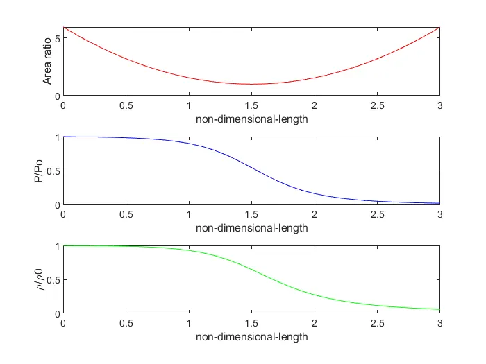
Plots for Non-Conservative-Form
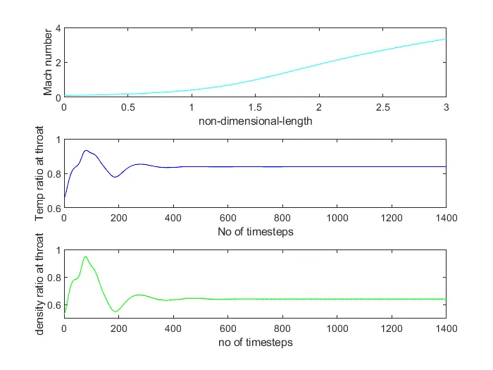
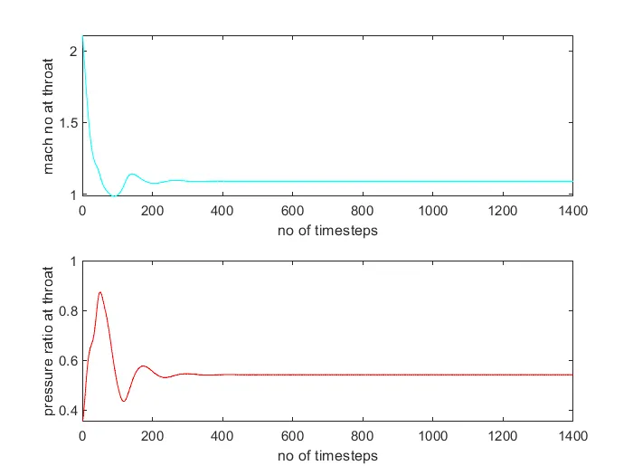
Time-wise variation of the primitive variables and mach number variation
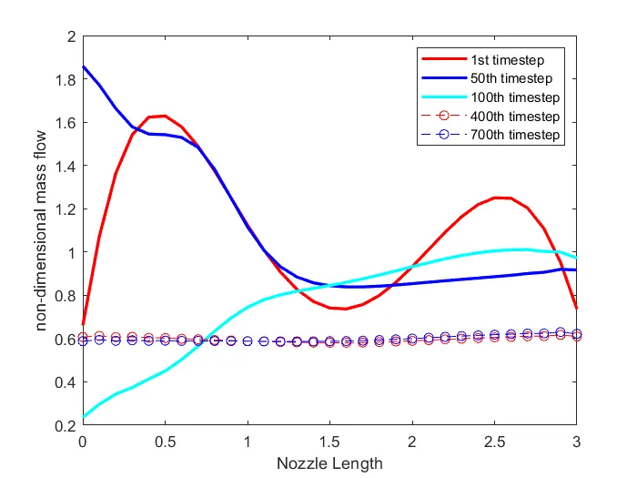
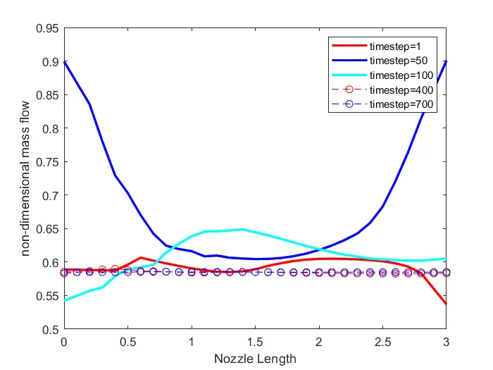
Variation of Mass flow rate distribution inside the nozzle at different time steps during the time-marching process
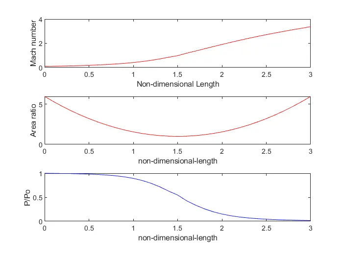
Plots for Conservative-Form
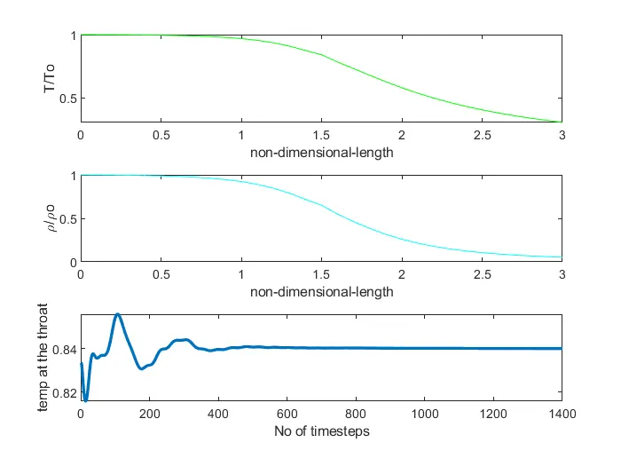
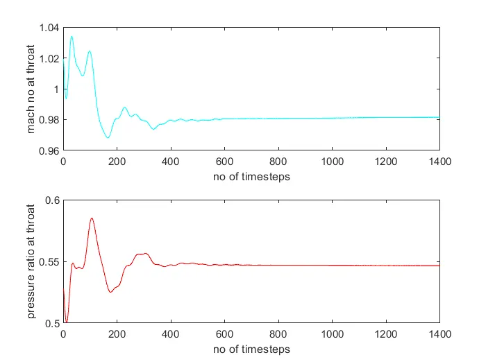
Time-wise variation of the primitive variables
Variation of Mass flow rate distribution inside the nozzle at different time steps during the time-marching process
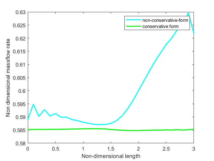
Comparison of Normalized mass flow rate distributions of both forms
COMPARISON OF CONSERVATIVE VS NON-CONSERVATIVE FORM
| PARAMETER | NON-CONSERVATIVE | CONSERVATIVE |
| VELOCITY AT THE EXIT | 1.8695 | 1.8660 |
| MACH NUMBER AT THE EXIT | 3.3496 | 3.3760 |
| TEMPERATURE AT NOZZLE EXIT | 0.3115 | 0.3055 |
| PRESSURE AT NOZZLE EXIT | 0.0174 | 0.0161 |
| DENSITY AT NOZZLE EXIT | 0.0559 | 0.0527 |
(NOTE: All the parameters are in their dimensionless form as stated in the formulation above)
GRID INDEPENDENCE STUDY
|
NO OF GRID POINTS/ PARAMETERS |
31 | 61 | 91 | Absolute error (in %) |
| VELOCITY AT THE EXIT | 1.8695 | 1.867 | 1.8692 | 0.1337 |
| MACH NUMBER AT THE EXIT | 3.3496 | 3.3563 | 3.3630 | 0.1996 |
| TEMPERATURE AT NOZZLE EXIT | 0.3115 | 0.3095 | 0.3089 | 0.642 |
| PRESSURE AT NOZZLE EXIT | 0.0174 | 0.0167 | 0.0165 | 1.2 |
| DENSITY AT NOZZLE EXIT | 0.0559 | 0.0541 | 0.0535 | 1.11 |
(NOTE: All the parameters are in their dimensionless form as stated in the formulation above)
Thus the nozzle flow is simulated and the conservative and non-conservative forms are discussed as usual.
The area ratio variation agrees with the theoretical variation as a function of x, and the pressure ratio, temperature ratio, and density ratio decrease because of flow acceleration to supersonic speeds. In the case of time-bound variation of primitive parameters, the parameters at the throat are plotted as a function of timesteps. We can infer from the above plots that after 200 timesteps, the solution converges to a steady state solution. The grid independence study is conducted so as to make sure that the solution remains approximately the same after varying the number of grid points.
EFFECTS OF COURANT NUMBER
Varying the courant number above the value of 1 causes the solution to become unstable. Hence the courant number effect is verified.
| Courant number | Velocity |
| 0.5 | 1.8695 |
| 0.7 | 1.8746 |
| 0.9 | 1.8819 |
| 1.5 | becomes unstable |