Week 6 - Multivariate Newton Rhapson Solver

Aim

To solve the following set of equations as mentioned below by using multivariate newton raphson method and assuming appropriate initial conditions.

Theory

The Newton-Raphson method (also known as Newton's method) is a way to quickly find a good approximation for the root of a real-valued function `f(x)=0`. It uses the idea that a continuous and differentiable function can be approximated by a straight line tangent to it.

Suppose you need to find the root of a continuous, differentiable function `f(x)`, and you know the root you are looking for is near the point `x=x_0`. Then Newton's method tells us that a better approximation for the root is

`x_1=x_0 - (f(x_0)/(f'(x_0)))`

This process may be repeated many times as necessary to get the desired accuracy. In general,for any `x`value `x_n`, the next value is given by

`x_(n+1)=x_n - (f(x_n)/(f'(x_n)))`

Note: the term "near" is used loosely because it does not need a precise definition in this context. However, x_0x0​should be closer to the root you need than to any other root (if the function has multiple roots).

Here is a picture to demonstrate what Newton's method actually does:

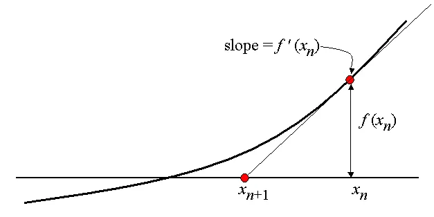
We draw a tangent line to the graph of `f(x)` at `x=x_0`. The line has slope `f'(x_n)` and goes through the point (`x_n,f(x_n)`). Therefore, it has the equation y=`f'(x_n)(x-x_n)+f(x_n)`. 

Now we find the root of this tangent line by setting y=0 and `x=x_(n+1)` for our new approximation . Solving this equation gives our new approximation which is 

`x_(n+1)=x_n - (f(x_n)/(f'(x_n)))`

Limitations of Newton-Raphson(NR) method

Newton's method may not work if there are points of inflection, local maxima or minima around `x_0` or the root. 

For example, suppose we need to find the root of `27x^3-3x+1=0`, which is near 0.

The correct answer is -0.44157265. However, NR method will give us the following values:

This is very clearly not helpful. That's because the graph of the function around x=0 looks like this:

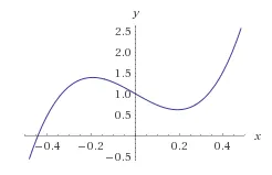
As you can see, this graph has a local maximum, a local minimum and a point of inflection around x = 0. To see why Newton's method isn't helpful here, imagine choosing a point at random between x = -0.19 and x = 0.19 and drawing a tangent line to the function at that point. That tangent line will have a negative slope, and therefore will intersect the y-axis at a point that is farther away from the root.

In a situation like this, it will help to get an even closer starting point, where these critical points will not interfere.

Now in this challenge, the given equations are 

• `(dy_1)/(dt)=-0.04y_1+10^4y_2y_3`
• `(dy_2)/(dt)=0.04y_1-10^4y_2y_3- 3*10^7y_2^2`
• `(dy_3)/(dt)=3**10^7y_2^2`

We are going to employ implicit euler method by assuming the initial condition as 1 for y1 and 0 for y2 and y3, taking alpha as 1.

To convert the above equation into a function, we will use implicit method i.e.

• `y_1^n=y_1^(n-1)+h**(-0.04*y_1^n+10^4y_2^ny_3^n)`
• `y_2^n=y_2^(n-1)+h**(0.04*y_1^n-10^4y_2^ny_3^n-3*10^7y_2^2)^n`
• `y_3^n=y_3^(n-1)+h**(3**10^7y_2^2)^n`

Once we bring all the equations to one side, then we can implement Multivariate NR method

• The logic is that  
  • First, we create three functions that contain three equations needed to be calculated
  • Then, a jacobian matrix is created which computes the jacobian matrix numerically as posed by the challenge
  • Then, a time array is created to indicate the number of times the solution has to run.
  • The timestep size is varied accordingly to see whether we get any change in the solutions
  • We import numpy for using commands like linspace, arange, etc.
  • We import matplotlib to plot graphs.
  • We use a while loop so that the solution runs until it converges.

Code

''' To solve the equation 
	dy1/dt=-0.04y1 +10^4y2y3
	dy2/dt=0.04y1-10^4y2y3 - 3*10^7y2^2
	dy3/dt=3*10^7*y2^2
	formula is x_new=x_old-alpha*inv(J)*f
	The above three equations are non linear
''' 

import numpy as np
from numpy.linalg import inv
import math
import matplotlib.pyplot as plt

#defining the equations 
def f1(y1_old,y1,y2,y3,h):
	return y1_old + h*(-0.04*y1 + (10**4)*y2*y3) - y1

def f2(y2_old,y1,y2,y3,h):
	return y2_old + h*(0.04*y1 - (10**4)*y2*y3 - 3*(10**7)*(y2**2)) - y2

def f3(y3_old,y1,y2,y3,h):
	return y3_old + h*((3*(10**7)*(y2**2))) -y3

def jacobian(y1_old,y2_old,y3_old,y1,y2,y3,h):

	#Numerically evaluating jacobian
	#jacobian matrix
	J=np.ones((3,3))
	dy=1e-4

	#First Row
	J[0,0]=(f1(y1_old,y1+dy,y2,y3,h)-f1(y1_old,y1,y2,y3,h))/dy
	J[0,1]=(f1(y1_old,y1,y2+dy,y3,h)-f1(y1_old,y1,y2,y3,h))/dy
	J[0,2]=(f1(y1_old,y1,y2,y3+dy,h)-f1(y1_old,y1,y2,y3,h))/dy

	#Second Row
	J[1,0]=(f2(y2_old,y1+dy,y2,y3,h)-f2(y2_old,y1,y2,y3,h))/dy
	J[1,1]=(f2(y2_old,y1,y2+dy,y3,h)-f2(y2_old,y1,y2,y3,h))/dy
	J[1,2]=(f2(y2_old,y1,y2,y3+dy,h)-f2(y2_old,y1,y2,y3,h))/dy

	#Third Row
	J[2,0]=(f3(y3_old,y1+dy,y2,y3,h)-f3(y3_old,y1,y2,y3,h))/dy
	J[2,1]=(f3(y3_old,y1,y2+dy,y3,h)-f3(y3_old,y1,y2,y3,h))/dy
	J[2,2]=(f3(y3_old,y1,y2,y3+dy,h)-f3(y3_old,y1,y2,y3,h))/dy

	return J


y_old=np.zeros((3,1))
y_old[0]=1
y_guess=np.zeros((3,1))
y_guess[0]=y_old[0]
y_guess[1]=y_old[1]
y_guess[2]=y_old[2]

alpha=1

t=np.linspace(0,10,601)
print(t)
dt=t[1]-t[0]
h=dt

f=np.copy(y_guess)
iterr=1
y1_solution=[]
y2_solution=[]
y3_solution=[]

for i in range(0,len(t)):
	tol=1e-16
	error=9e9

	while error>tol:
		J=jacobian(y_old[0],y_old[1],y_old[2],y_guess[0],y_guess[1],y_guess[2],h)

		f[0]=f1(y_old[0],y_guess[0],y_guess[1],y_guess[2],h)
		f[1]=f2(y_old[1],y_guess[0],y_guess[1],y_guess[2],h)
		f[2]=f3(y_old[2],y_guess[0],y_guess[1],y_guess[2],h)

		y_new=y_guess- alpha*np.matmul(inv(J),f)

		error=np.max(np.abs(y_new-y_guess))

		y_guess=y_new
	y_old=y_new
	y1_solution.append(y_new[0])
	y2_solution.append(y_new[1])
	y3_solution.append(y_new[2])
print(y1_solution,y2_solution,y3_solution)
plt.plot(t,y1_solution,label='Y1')
plt.plot(t,y2_solution,label='Y2')
plt.plot(t,y3_solution,label='Y3')
plt.legend()
plt.show()

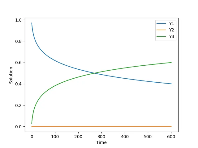
For timestep size of 1

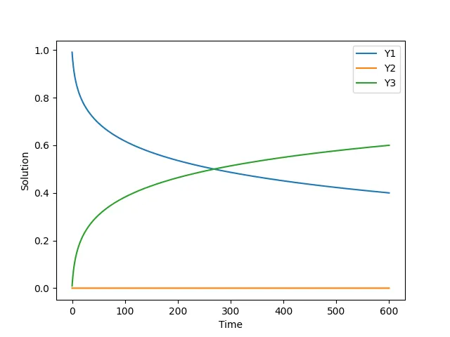
For timestep size of 0.5

For timestep size of 0.25

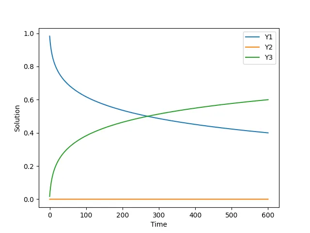
• The above graphs shows the values of the three unknowns y1,y2 and y3.
• Note that in the above graphs, the value suddenly changes and then attains steady state. 
• It is important to note that as the timestep size varies, there is little to no variation in the solution as the timestep size decreases and hence the solution becomes stable because of the implicit method that is used.
• For an implicit method, we dont have to choose a particular step size i.e. this method is unconditionally stable and hence the time step size selection is irrelevant in this case. 
• If the solution were executed based on explicit scheme, the solution can quickly go unstable because of stability criterion being imposed on the system of equations and on the timestep size.

Thus the Newton-Raphson method is studied and the code is written.