Week 5: Prandtl Meyer Shock problem
Prandtl Meyer Shock problem
In this simulation, we will understand what a shock is (expansion fan) and understand its significance in the flow properties alterations. Also, we will
-
Do a literature search on what BC's are typically used for shock flow problems
-
We will understand what is a shock wave. In your own words, describe the physics behind shock waves
-
- Effect of SGS parameter on shock location
- In the Prandtl Meyer shock problem, we shall look at the effect of SGS temperature value on cell count and the shock location
Introduction
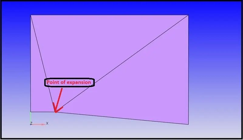
A shock is a propagating wave that travels through a medium,typically of the order of 10`mu`m thickness, across which drastic flow properties (change is temperature, pressure) happen.Shock may also be described as a front in a supersonic flow field, and the flow processing across the front results in an abrupt change in fluid properties. In other words, shock is a thin region where large gradients in temperature, pressure, and velocity occur and where the transport phenomena of momentum and energy are important.The thickness of the shocks is comparable to the mean free path of the gas molecules in the flow field. Note that when flow is suddenly expanded, an expansion fan is generated at the point of expansion. To understand this, consider a schematic representation of shock as shown below.
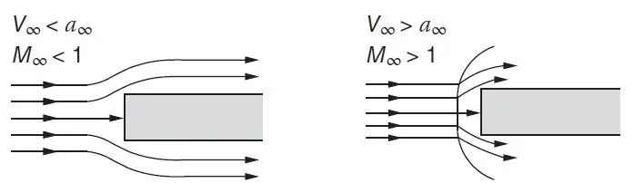
We know from kinetic theory that the flows consist of a large number of fluid molecules in unit volume and the transport ofmass, momentum, and energy takes place through the motion of these molecules. Also, the molecules carry the signals about the presence of the cylinder around the flow field at a speed equal to the speed of sound. In the above figure, the incoming stream is subsonic, V∞<a∞ and the molecules far upstream of the cylinder get information about the presence of the cylinder through the signals which travel with speed a∞, well before reaching the cylinder. Therefore, the molecules orient themselves in order to flow around the cylinder, as shown in figure. But when the incoming stream is supersonic, the molecules travel faster than the signals and there is no possibility that they will be informed of the presence of the cylinder before they reach it. Also, the reflected signals from the cylinder face tend to coalesce at a short distance ahead of the cylinder.Their coalescence forms a thin compression front called a shock wave, as shown in Figure 3.1b. Upstream of the shock, the flow has no information about the presence of the cylinder. However, the streamlines behind the shock quickly compensate for the obstruction, since the flow is subsonic after a detached shock, as shown in the figure. Although the shock formation discussed above is for a specific situation, the mechanism described is, in general, valid. However, we should realize that, when the flow just starts, there is no shock. The formation of shock takes place after the fluid molecules impinge on the cylinder face and rebound.
Note: This project corresponds to that of a prandtl-meyer expansion fan,not a shock wave.
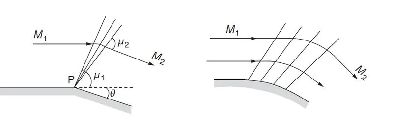
Note that the geometry attached below is similar to the above. Since a supersonic flow when subjected to a convex corner, expansion fans are generated which increase the flow mach number while the shock wave decreases it. This is an important criterion to be noted while discussing the differences between expansion fan and a shock wave.
Shock flow Boundary conditions
When solving the Navier-Stokes equation (i.e. the fluid’s governing equations) and continuity equation, appropriate initial conditions and boundary conditions need to be applied. Various types of boundary conditions will be discussed in more detail in this challenge.
Neumann and Dirichlet Boundary Conditions
• When using a Dirichlet boundary condition, one prescribes the value of a variable at the boundary, e.g.


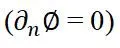
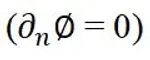
• When using a Neumann boundary condition, one prescribes the gradient normal to the boundary of a variable at the boundary, e.g.


Inlet
Inflow
• Transported variables specified on the boundary, either by a predefined profile or (user’s preference) by doing an initial 1D, fully-developed-flow calculation.
Stagnation (or reservoir)
• Total pressure and total temperature (in compressible flow) or total head (in incompressible flow) fixed; usual inflow condition for compressible flow.
Outlet
Outflow
• Zero normal gradient for all variables.
Pressure
• As for outflow, except fixed value of pressure; usual outlet condition in compressible flow if the exit is subsonic.
Symmetry
• Symmetry boundary conditions are those that arise by viewing the computational domain as a sub-region of some larger domain which possesses planes or axes of symmetry.
• In a typical CFD code, plane two-dimensional flows can be simulated using a single layer of cells bounded on its sides by symmetry planes, since there is no velocity component in the spanwise direction.
• Symmetry boundary condition can also be applied to axially symmetric flows, for instance by generating a single segment of cells and applying the symmetry conditions on the segment surfaces.
• Applying symmetry boundary conditions can significantly reduce the mesh size and consequently results in considerable savings in computational time.
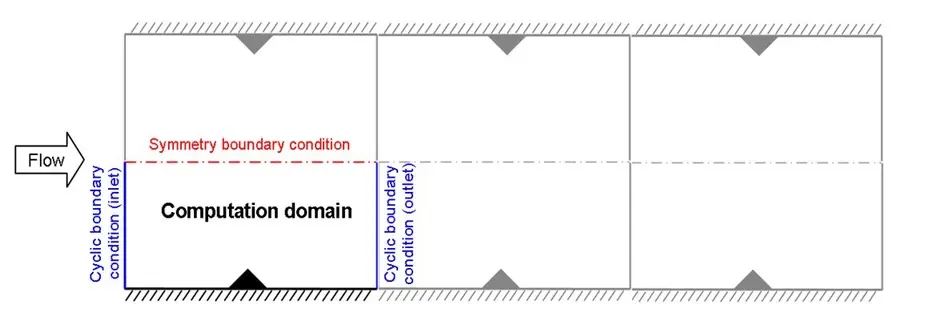
Periodic (Cyclic)
• This type of boundary condition consists of pairs of geometrically identical boundaries at which all flow conditions are matched.
• A simple example is that of a 2D channel with both walls roughened by a repeating obstacle.
• By using symmetry and cyclic boundary conditions, it is possible to solve only a small section made up of one symmetry plane and one pair of cyclic boundary conditions.
• In applying periodic boundary conditions, special treatment of the transport equations is required: by adding extra source terms to the momentum and energy equations, the streamwise pressure drop and temperature increase due to heating are accounted for.
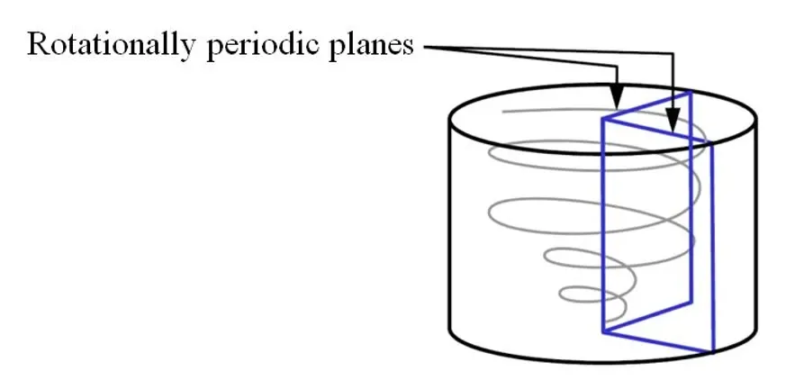
Rotational Periodicity
• ΔP = 0 across periodic planes.
• Axis of rotation must be defined in fluid zone.
• Translational periodicity.
• ΔP can be finite across periodic planes.
• Models fully developed conditions.
• Specify either mean ΔP per period or net mass flow rate.
Wall Boundary Conditions
• Wall boundaries can be defined as no-slip or slip walls
• In viscous flows, no-slip conditions are applied at walls.
• The wall thermal boundary conditions are usually defined as constant temperature or constant heat flux.
• Special treatments are available to represent wall roughness.
Procedure
In this project, we will work on generation of expansion fan and try to simulate the velocity and pressure contours using converge CFD.
- At first, the model is imported into the converge studio
- Then the boundaries are flagged as inlet , outlet , top and bottom walls, front and back face
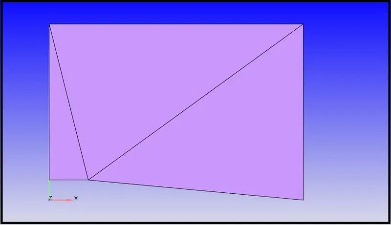
- Note that we are simulating 2-D case, hence the top and bottom walls can be treated as a 2-D boundary condition.
- Once done, lets begin case setup.
- In case setup, choose steady state mode of operation.
- Setup the simulation time parameers. The simulation is run for 25000 cycles. Once done, we shall setup the boundary conditions.
- A region is initialized with a velocity of 680m/s
- In the boundary conditions, the following boundaries are setup
- Inlet->Supersonicc BC with an inlet velocity of 680 m/s(Mach 2) with a pressure BC of zero normal gradient
- Outlet->Both velocity and pressure BC are set to zero normal gradient
- Wall->Slip boundary conditions
- Front and back face->2-D
- Once done, choose the physical model as turbulence RNG k-e model
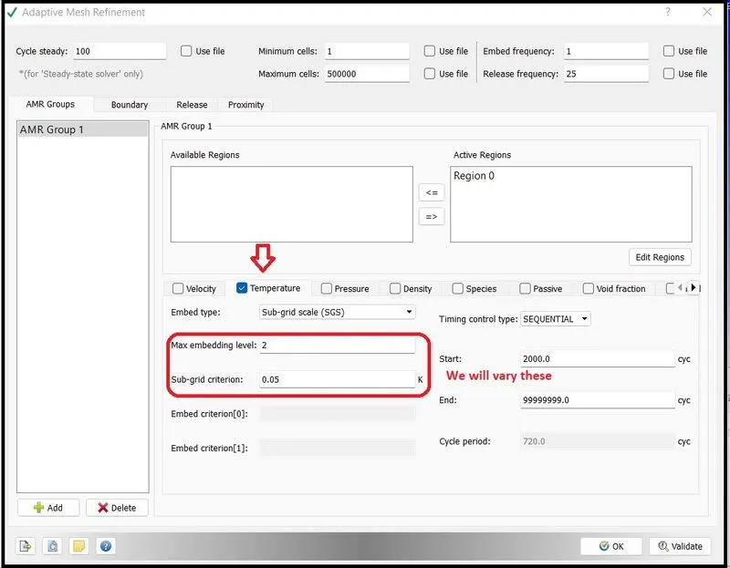
- Next step is to choose Adaptive mesh refinement.
- Once done, choose the base mesh size as 0.8m(First scale down the model in m, and then apply this size).
- Once done, export the input files to a folder.
- Open cygwin and run the solution.
- Once the solution converges, post-convert the solution so that the results can be visualised in paraview.
- It is also necessary to view the line plotting solution of parameters like mass flow rate, velocity,etc.
Results and Discussions
Here we consider an SGS factor of 0.05 and 0.1 for comparison purposes.
-> With an SGS of 0.05K
Animations of
| Par | SGS of 0.05K | SGS of 0.1K |
| Velo. | ||
| Pres. | ||
| Temp. |
Plots showing variation of parameters along the length of the contour
| SGS of 0.05K | SGS of 0.1K | |
| Temp | 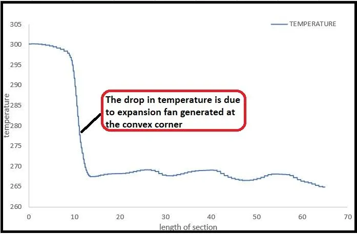 |
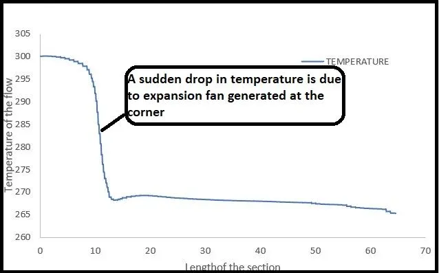 |
| Press | 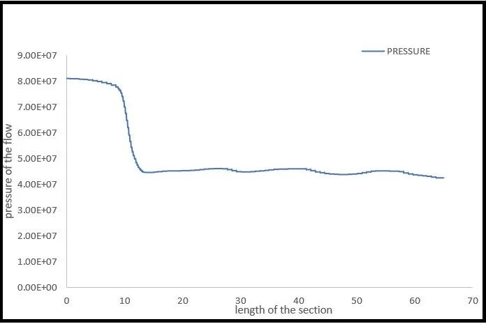 |
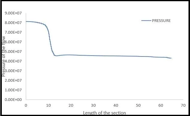 |
| Velo | 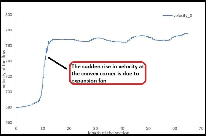 |
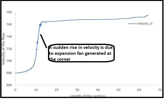 |
- Noting from the above chart that the temperature and pressure drops whereas the velocity increases suddenly at the point of expansion.
- This is due to the fact that when a supersonic flow is turned away from itself, a centered expansion fan is generated which accelearates the flow whilst the static temperature, static pressure and density decrease and the flow mach number is accelerated.
- But also note that the total properties like total temperature, total pressure remains constant since an expansion fan is an isentropic process
- (an isentropic process is one in which the flow is reversible as well as adiabatic)
- To understand the difference between total and static properties, imagine that you are travelling along with the flow. The properties that you measure as you move along with the flow is called static property
- Imagine that the flow moving at some speed is slowed down to zero velocity isentropically. Then the flow properties are called total properties.
Comparison of plots
| SGS of 0.05K | SGS of 0.1K |
 |
 |
 |
 |
 |
 |
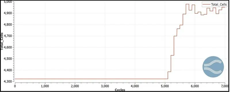
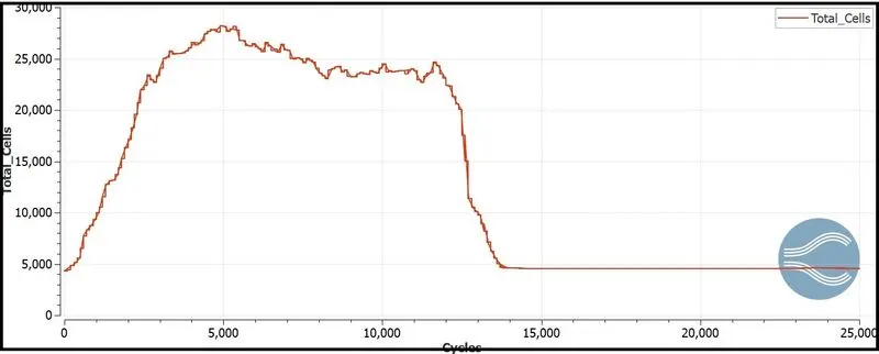
- The first plot depicts variation of no of cells as the no of cycles increases.
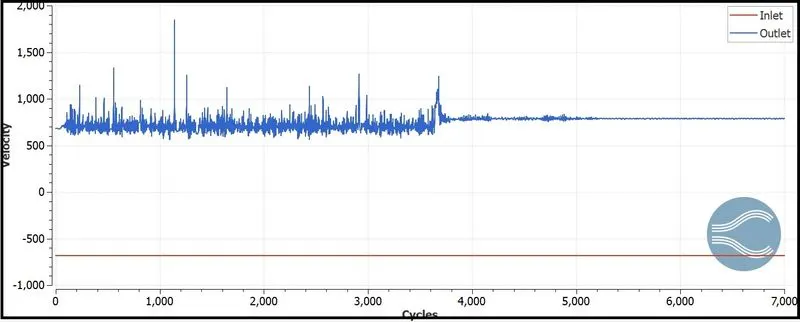
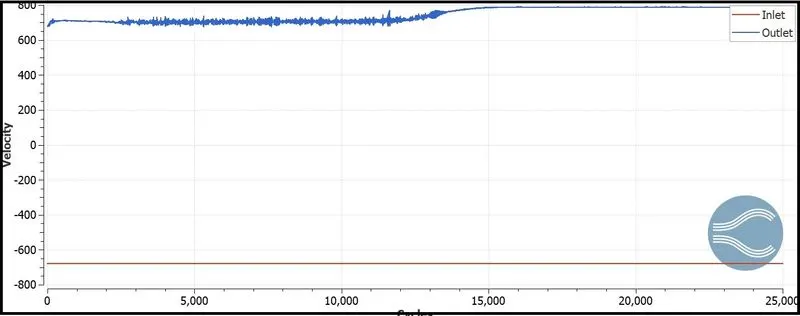
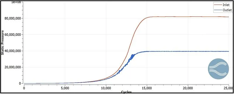
- The second plot shows Convergence of velocity after a number of iterations.
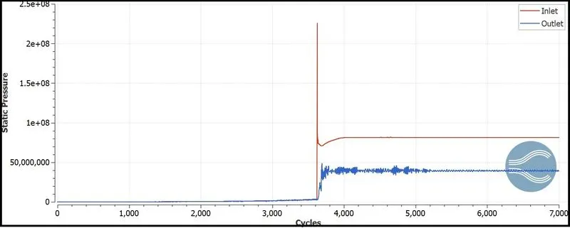
- The third plot shows Convergence of pressure after a number of iterations.
- Here, we can note that the velocity converges after 4000 cycles.
- While the inlet velocity remains constant, it is the outlet velocity that fluctuates as the expansion fan creates some unsteadiness initially.
- Note that a negative value corresponds to an inflow condition(flow is entering the control volume) whereas the positive value corresponds to an outflow condition(flow is leaving the control volume).
- Hence the outlet velocity is higher than the inlet velocity(magnitudes only)
- Here, we can note that there is a sudden spike in pressure value.
- Both the inlet and outlet pressure fluctuates as the expansion fan creates some unsteadiness initially.
- Note that because of the expansion fan, there is a drop in pressure at the outlet.
- Hence the static pressure at the outlet is smaller than that of inlet.
- As we can see, the number of cells almost remain constant, then show a sudden stepwise variation. This is due to AMR(adaptive mesh refinement).
| AMR(adaptive mesh refinement) | 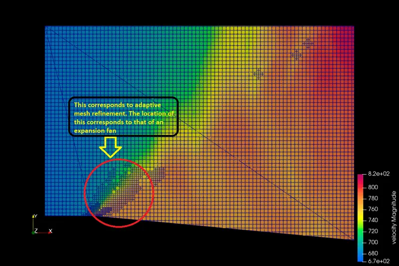 |
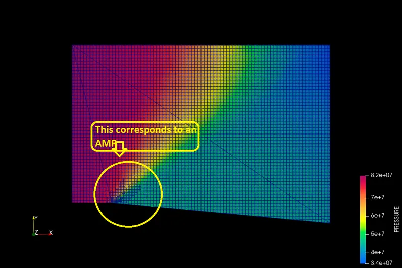 |
- Note that because of adaptive mesh refinement(AMR), we get sub grid mesh sizes of size half of that of the original mesh grid size.
- Note that they occur only at the point of generation of expansion fan because drastic changes happen to the flow properties across an expansion fan.
- This corresponds to a subgrid size of 0.05
Let `underset(o)(P),underset(o)(T)` denote total pressure and total temperature respectively. Then across an expansion fan, the following happens.
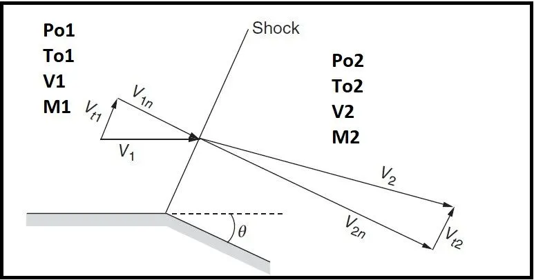
Let 1 be the region ahead of the expansion fan and let 2 be the region behind the expansion fan. Then across an expansion fan, the following happens:
`underset(2)(V)>underset(1)(V)`
`underset(1)(P)>underset(2)(P)`
`underset(1)(T)>underset(2)(T)`
`underset(01)(T)=underset(02)(T)`
`underset(01)(P)=underset(02)(P)`
SGS study comparison
| Parameter | with SGS of 0.05K | with SGS of 0.1K |
| Temperature(in K) | 264.897 | 265.242 |
| Pressure(in Pa) | 4.27e+07 | 4.31e+07 |
| Velocity(in m/s) | 778.391 | 777.97 |
The effect of SGS isnt much predominant while varying the factor by two. Infact both the values are very close to each other.
Thus the prandtl-Meyer expansion fan is simulated and comparisons have been drawn.