Week 5 - Rayleigh Taylor Instability
Challenge
In this challenge, Rayleigh taylor instability simulation is performed for 2 different mesh sizes and an extra simulation with a user defined material incorporated in fluent. The following tasks are carried out in this challenge:
1. To compare the results by showing the animations of all the cases.
2. To observe the differences in the animation and explain the effect of mesh size on simulation.
3. To explain why a steady-state approach might not be suitable for these types of simulation.
4. To define the Atwood Number and to find out the Atwood number for both the cases and explain how the variation in Atwood number in the above cases affect the behavior of the instability.
Rayleigh Taylor Instability(RTI):
Rayleigh-Taylor instability (RTI) is the interpenetration of materials that occurs whenever a light fluid pushes on a heavy fluid. It is a dynamic process whereby the two fluids seek to reduce their combined potential energy. The ensuing turbulence and mixing has far-reaching consequences in many natural and man-made flows, ranging from supernovae to inertial confinement fusion (ICF) capsules to mushroom clouds formation in nuclear detonation,etc.
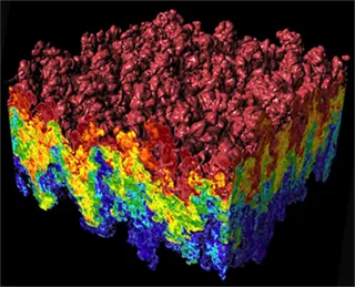
RT instability exits in many situations from overturn of the outer portion of the collapsed core of a massive star to laser implosion of deuterium-tritium fusion targets. In the mixture of fluids, the instability is triggered by the gravitational force acting on an inverted density gradient.
CFD models based on RTI:
1. VOF(Volume of Fluid)
It is a free surface modeling technique for tracking and locating the free surface or fluid-fluid surface. It belongs to the class of Eulerian mechanics which are characterized by a mesh that is stationary or moving in a certain prescribed manner.
2. k-L turbulence model
The k-L model was proposed by Dimonte and Tioton for describing the turbulent self similar regime of RT and RM induced mixing. The model describes the dominant eddies in the mixing zones with evolutionary equations for their characteristic dimension
3. Kelvin-HelmHoltz model
This model was used to predict the primary breakup of the intact liquid core of the jet and this model determines the effect of acceleration of the different phases.
Procedure:
The process involves creating a surface in spaceclaim.
The next step is to mesh the surface. Here we perform a base mesh of 0.5 mm and a refined mesh of 0.1 mm to capture the pattern and to check whether the pattern varies.
This is followed by setting up the solver and applying laminar viscous model.
Since the domain involves two fluids, we consider VOF(volume of fluid approach). We patch the regions and initialise the domain and then solve for a number of iterations.
Geometry Creation:
We consider two squares of 20mm*20mm and one surface will contain air and the other surface will contain water. The motive is to observe the instability when fluid mixes under the effect of gravity. Name one surface as air and the other surface as water. Click on share button in the workbench tab which will detect the common surface between two surfaces.
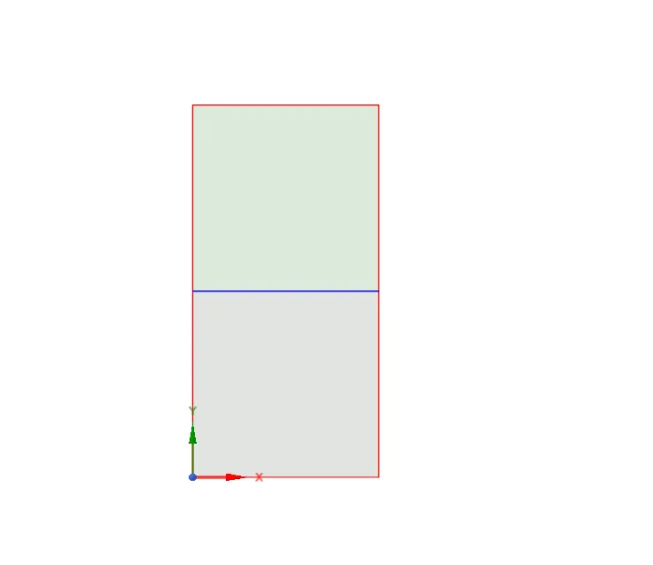
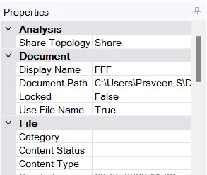
Once done, we will be able to see share option under shared topology. Close the spaceclaim and open meshing.
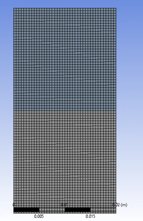
In meshing, click on face meshing and size it to 0.5mm. This will serve as our base mesh. Once that is done, update the mesh and close meshing.
Open Fluent solver and the first process is to select the viscous model as laminar model.
Next click on multiphase and click on VOF. Select the analysis to implicit.
Next go to phases and make air as the primary phase and water as secondary phase.
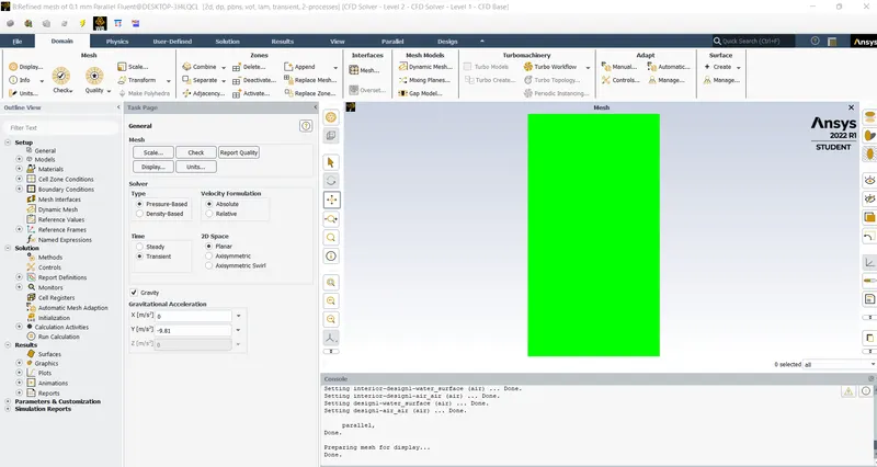

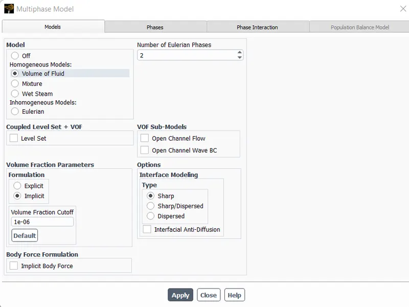
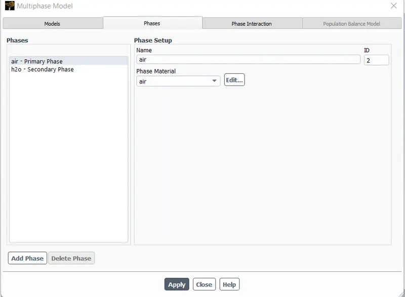
Once done, go to solutions and initialise. Then click on patch and give the value of 1 for water component and 0 for air component and run the solution for a number of iterations.
Case 1: When mesh size is 0.5 mm
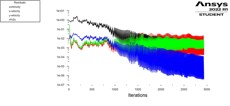
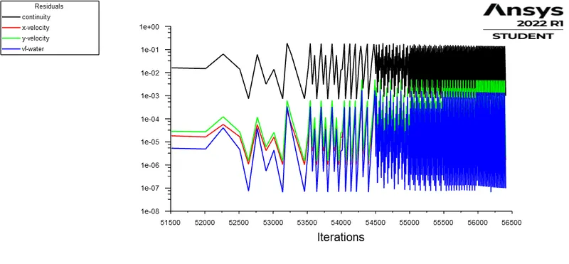
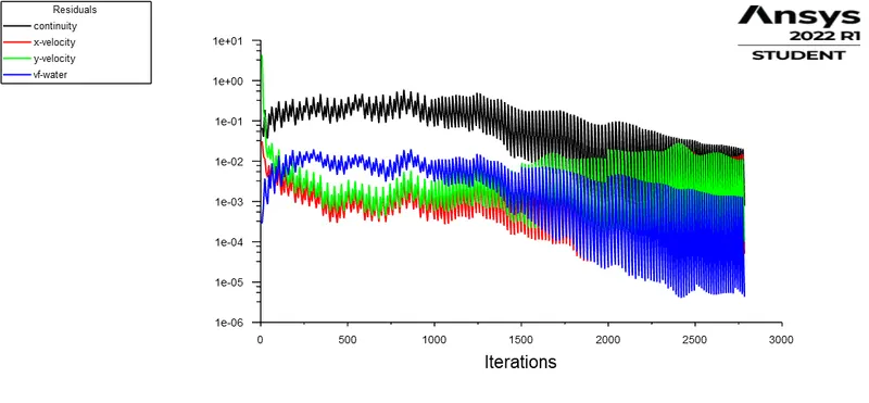
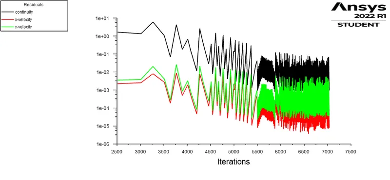
Convergence of solution-oscillations in transient case
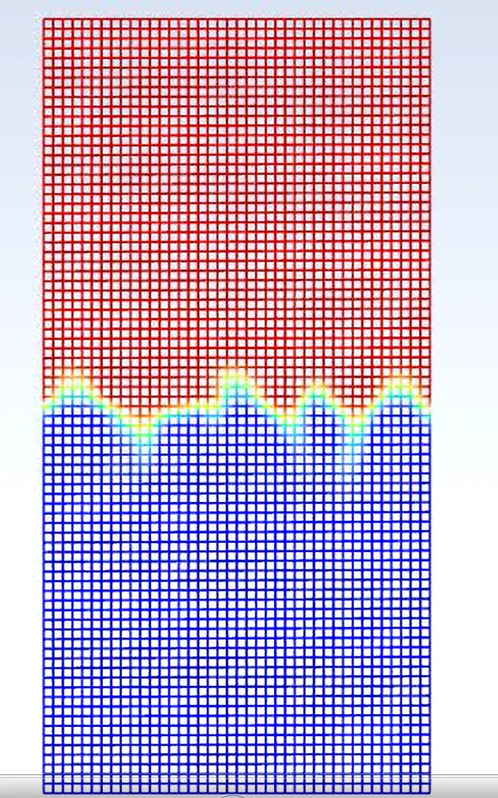
Pattern of formation of bubbles for a mesh size of 0.5 mm
Case 2: when mesh size is 0.1 mm
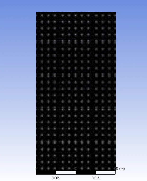
The difference between the above two cases are the formation of drops and instability patterns is a bit more appealing,but it takes a lot of time to actually get the accurate solution for a large number of iterations. We are also able to get a clear plot of mixing of fluids whilst the effect of gravity is predominant. With increasing mesh sizing, we get better visualization and the cons is that the time taken to converge for the refined mesh is very large.
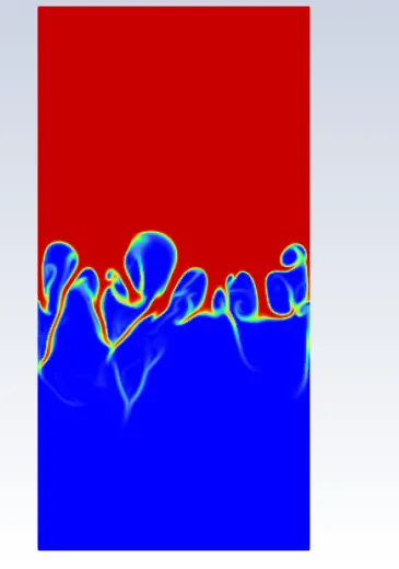
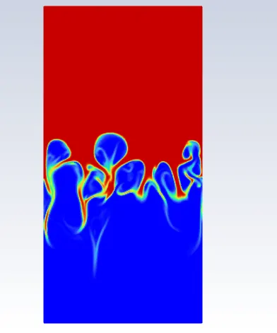
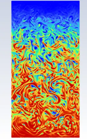
This visualisation pattern is non evident in the baseline mesh.
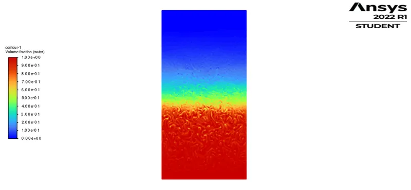
Case 3: (with a user defined material of density 400 kg/m^3 and viscosity 0.001 kg/ms)
base mesh of 0.5mm
In this step, we have to create a new material in place of air by using create material option in fluent. We use the base mesh size of 0.5 mm and creating a new material in place of air whose density and viscosity values are specified. The remaining procedure needs to be followed as same.
with refined mesh of 0.1 mm, it looks like
Steady analysis:
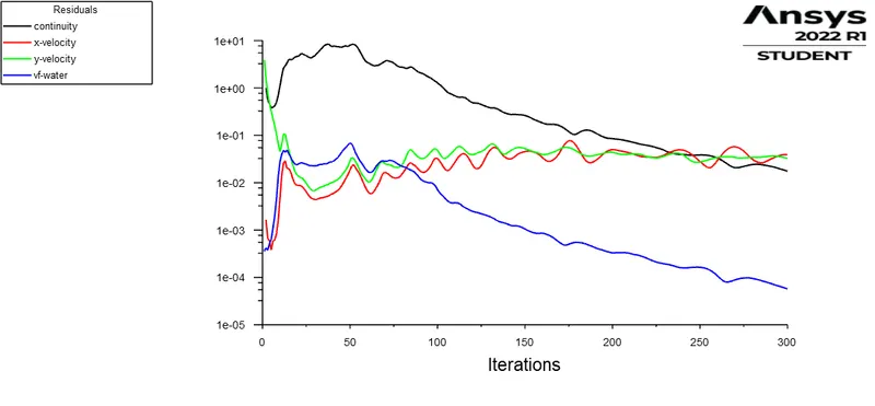
It is evident from the above video that a steady analysis misses out in providing key contours like the formation of bubbles and mixing and hence it is not suitable for instability analysis. Because in a steady state, we are ignoring time derivatives which causes the solution to simplify a lot.
Atwood Number
Atwood number is defined as `At=(rho1-rho2)/(rho1+rho2)`
where `rho1`-> density of heavier fluid
`rho2`-> density of lighter fluid
Atwood number is a dimesionless number in fluid dynamics used in the study of hydrodynamic instabilities in density stratified flows. It is an important parameter in the study of rayleigh taylor instability. In rayleigh taylor instability, the penetration distance of heavy fluid bubbles into the light fluid is a function of acceleration time scale`A*g*t^2`, where g is the gravitational acceleration and t is the time.
Atwood number for air and water case is
`underset(air)(rho)=1.225 (kg)/m^3` `underset(water)(rho)=998(kg)/m^3`
At=0.99755
Atwood number for udm(user defined material) and water is
`underset(water)(rho)=998 (kg)/m^3` `underset(udm)(rho)=400(kg)/m^3`
At=0.4285
When At ~1, due to large density difference, we can clearly see the patterns of bubble formation and distinct instability pattern.
When At<<1, due to small density difference, we cant see the instability clearly.