Week 6: Conjugate Heat Transfer Simulation

Conjugate Heat Transfer Simulation

In this simulation, we will setup a Conjugate heat transfer(CHT) analysis of flow through a solid pipe with a thickness and

• Setup a flow simulation through a pipe
• Inlet Reynolds number should be 7,000
• Add Y+ to your post.in file
• Start with an initial base grid
• Run grid dependence test on 3 grids and show that the outlet temperature converges to a particular value
• Set supercyle stage interval to 0.01,0.02 and 0.03
• For these three values, how does the total simulation time compare against the baseline configuration?
• Also create an animation and upload it on You tube and provide the You tube link for an animaion in the report.

Theory

Conjugate heat transfer is a type of heat transfer analysis between solids and fluid(s). This type of heat transfer includes both convection (between fluids) and conductive (between solids) heat transfer, as well as both forced and natural convection. Common applications and use cases of this thermal simulation type include electronics cooling, heat exchangers, industrial machinery,etc.

In most cases, heat transfer in solids, if only due to conduction is given by fourier's law of heat conduction which describes heat flux as `q=-knablaT`, whereas for a time-dependent problem, the temperature field in an immobile solid verifies the following form of the heat equation:

`rho*underset(p)(C)*(delT)/(delt)=nabla.(knablaT)+Q`

In a fluid, due to the fluid motion, three contributions to the heat equation are included:

1. The transport of fluid implies energy transport too, which appears in the heat equation as the convective contribution. Depending on the thermal properties on the fluid and on the flow regime, either the convective or the conductive heat transfer can dominate.
2. The viscous effects of the fluid flow produce fluid heating. This term is often neglected, nevertheless, its contribution is noticeable for fast flow in viscous fluids.
3. As soon as a fluid density is temperature-dependent, a pressure work term contributes to the heat equation. This accounts for the well-known effect that, for example, compressing air produces heat.

Heat transfer in fluids and solids can also be combined to minimize heat losses in various devices. Because most gases (especially at low pressure) have small thermal conductivities, they can be used as thermal insulators. In areas which involve cooling of components like turbine blades and transfer of heats across media, CHT is necessary to accurately model the system.

Procedure

The procedure involves first constructing a cylindrical pipe and providing a thickness and then flagging the boundaries followed by setting up the case by applying materials to solid pipe and applying BCs and then specifying the size of the mesh. The solution is then run in cygwin and postprocessed so that using paraview we can visualise the results.

• First, a geometry is constructed by specifying the inner radius of the cylinder as 0.015m and the radius of the outer cylinder as 0.02m.
• 
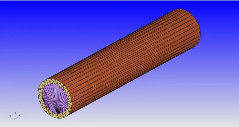
• Once done, the next step is to check whether any normal points out of the geometry. Next go to case setup and begin setting up the case.
• 
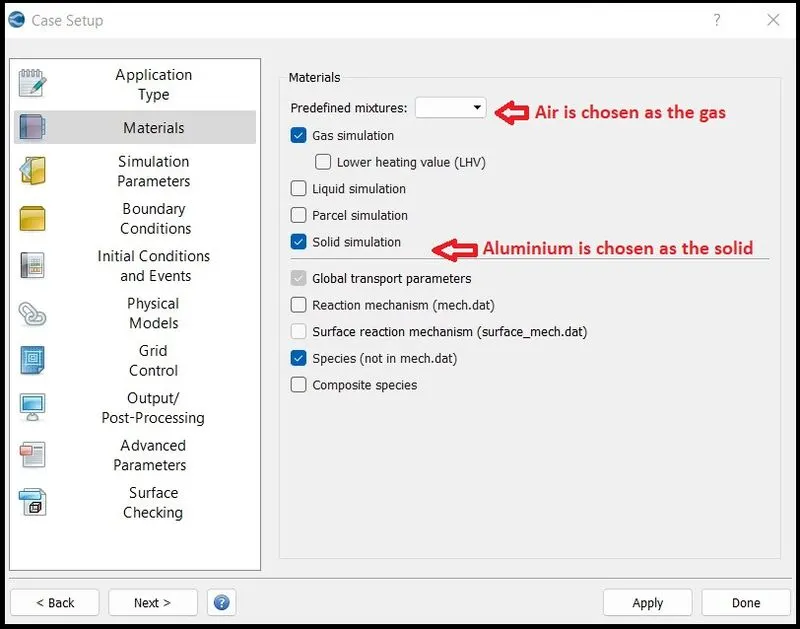
• Choose predefined mixture for gas as air and for solid as aluminium. We will be using these throughout the whole challenge. Turn on both gas and solid simulation.
• 
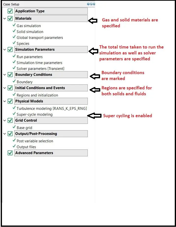
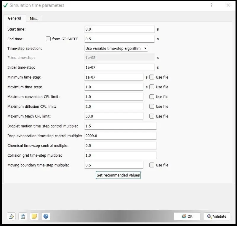
• The next step is to setup the simulation parameters. Set the mode of simulation as transient and specify the timestep size and the time taken to flow.
• 
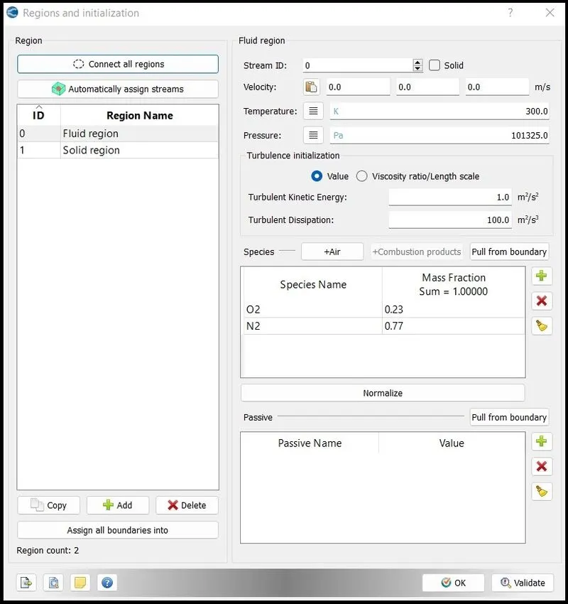
• Once done, the next step is to setup regions. Note that since we are simulating a CHT, we will be using two regions-one for fluid and one for solid.
• Note that while creating a region for solid, check the box'solid'so that the solver can understand it as another region
• Specify the materials in both the regions.
• Once done, we can setup the boundary conditions as follows
  • Note that we have five boundaries, so we specify inlet BCs as zero normal gradient and specifying inlet velocity as 3.413m/s(note that the reynolds number is 7000).
  • The outlet BC is specified as pressure specified region.
  • The solid outer wall is treated as a wall region and with a slip BC and a heat flux of -10kW/m^2
  • The interface region is applied and forward boundary is specified as fluid region and reverse boundary is specified as solid region
• 
• Setup super cycling for different supercyle stage interval to 0.01,0.02 and 0.03s respectively.
• In the output files, enable Y+ and export the input files to a desired folder.
• The procedure is repeated for different mesh sizes as well.

Results and Discussions

Meshgrid
Mesh size of 0.004m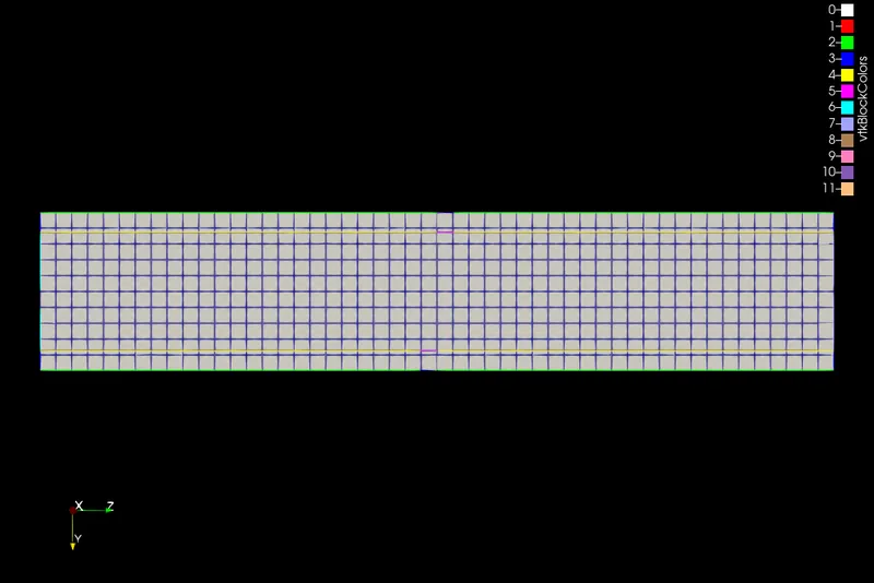
Mesh size of 0.002m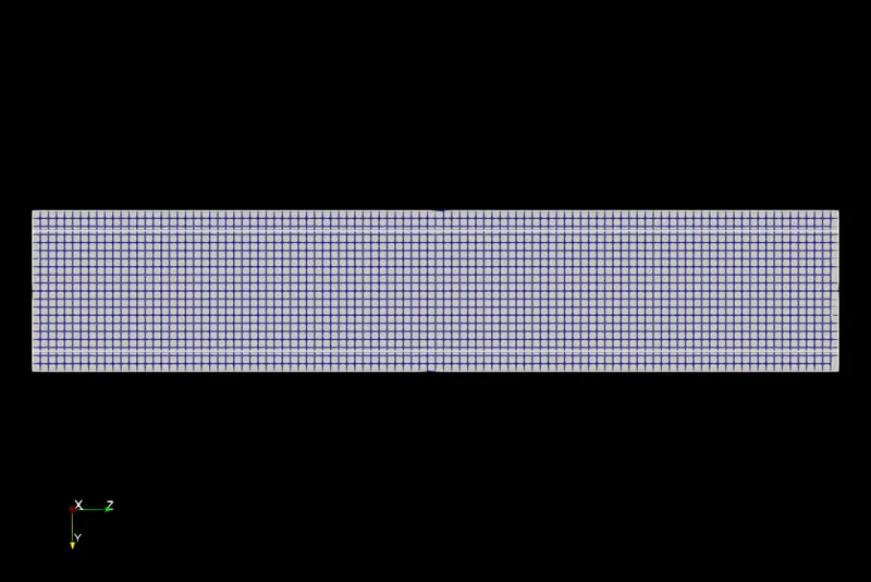
Mesh size of 0.0015m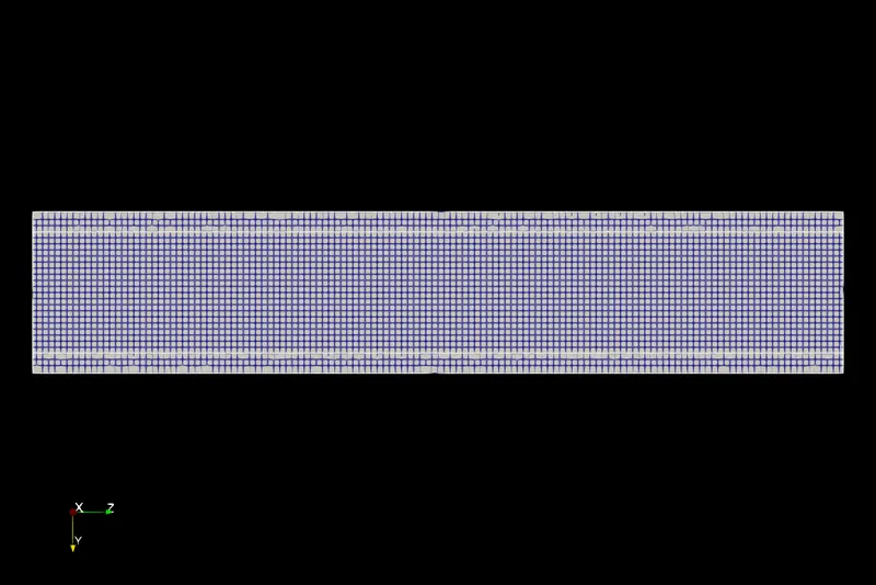

Contours of	Velocity
Mesh size of 0.004m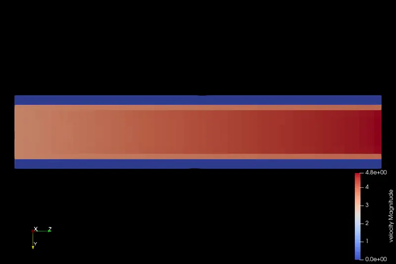
Mesh size of 0.002m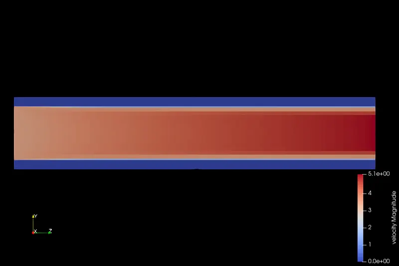
Mesh size of 0.0015m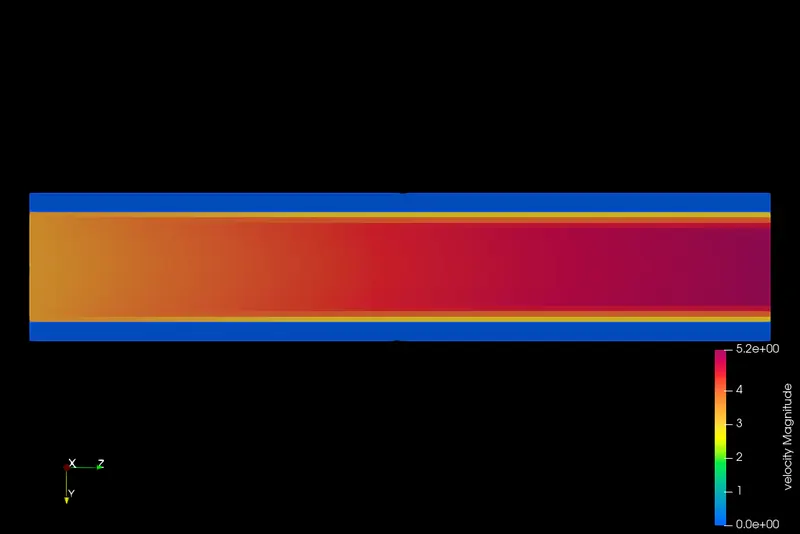

Contours of	Temperature
Mesh size of 0.004m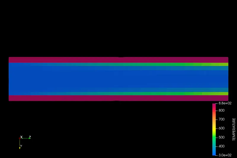
Mesh size of 0.002m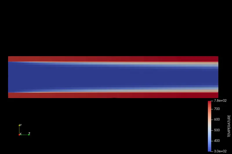
Mesh size of 0.0015m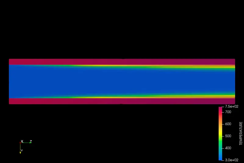

	Yplus
Mesh size of 0.004m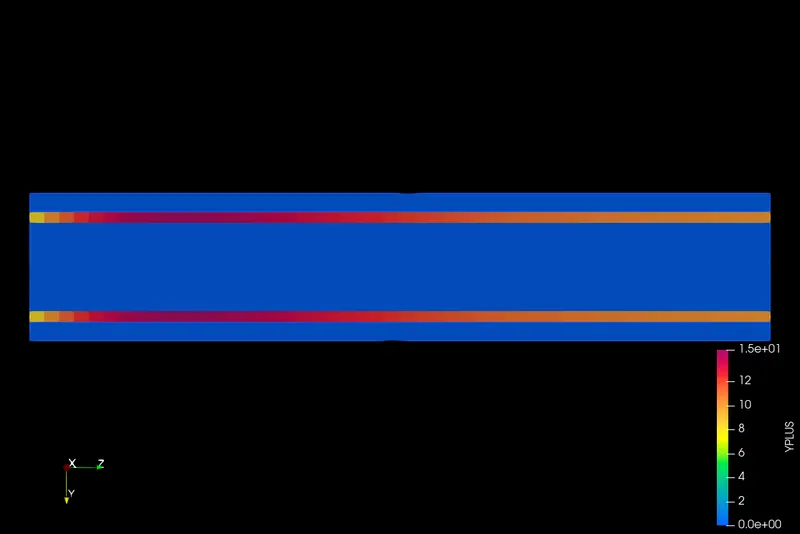
Mesh size of 0.002m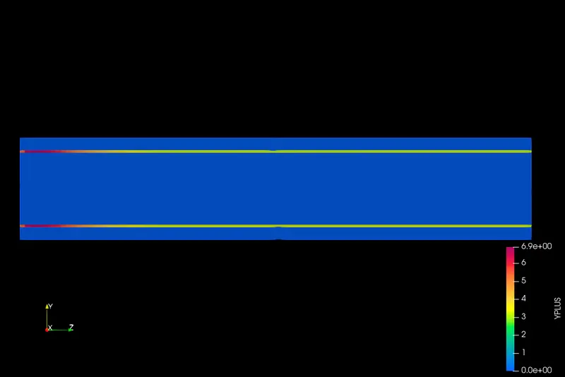
Mesh size of 0.0015m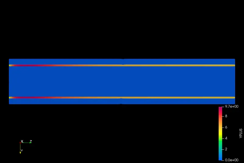

• The mesh size is shown above for different meshgrid sizes.
• Note that the no of elements increases as the size of the mesh decreases.
• Hence the time taken to run the solver will be longer for large number of cells
• The contours of velocity are shown above for all three different mesh sizes.
• Note that by reducing the mesh size, we get a better contour.
• At the inlet,the velocity appears same across the duct but at the exit, the velocity at the centre is larger than at the edge of the pipe.
• Also note that the velocity at the outlet is larger than that at the inlet because heat is added to the flow which increases the temperature of the fluid at the exit, which in turn increases the kinetic energy of the gas which inturn increases the exit velocity.
• As we can see from the above pics that better the mesh, better will be the distribution of temperature at the wall
• On further refining the mesh, we can see that the mesh affects the range of temperature.
• So ideally 0.002m or 0.0015m mesh size can be used so as to provide better values at the wall.
• By analysing the range of values of Y+ for three different mesh sizes, we can conclude that the mesh size of 0.002m is optimum mesh to capture details at the wall since the value of Y+ is <10.
• Y+ values lying in the range of 10 to 30 are difficult to capture and process data and hence the value of Y+ should be avoided in this region.

Characteristic plots

Parameters	mass flow rate
Mesh size of 0.004m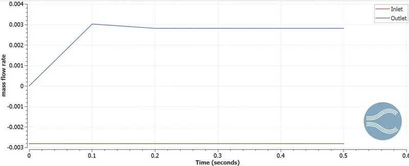
Mesh size of 0.002m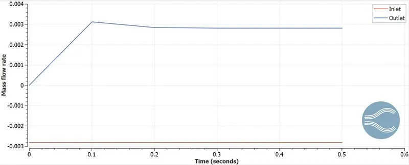
Mesh size of 0.0015m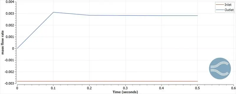

Parameters	Static pressure
Mesh size of 0.004m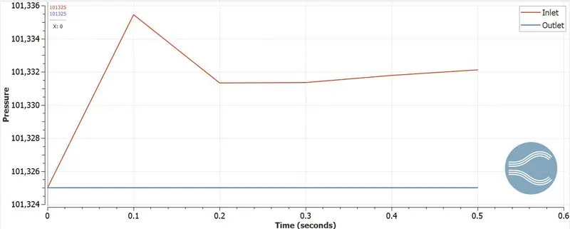
Mesh size of 0.002m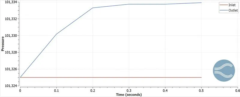
Mesh size of 0.0015m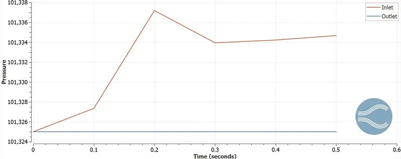

Parameters	Velocity
Mesh size of 0.004m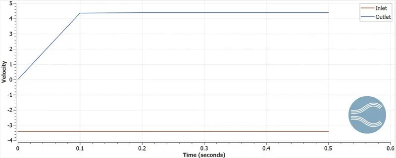
Mesh size of 0.002m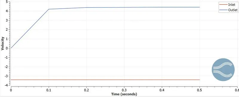
Mesh size of 0.0015m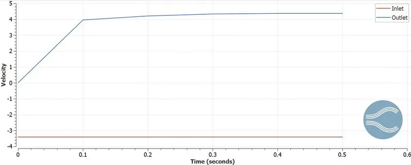

Parameters	Total cell count
Mesh size of 0.004m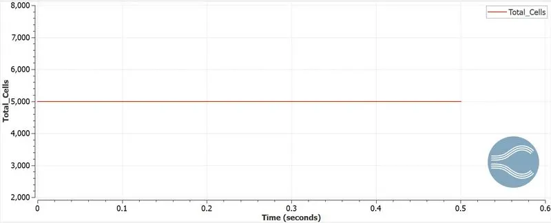
Mesh size of 0.002m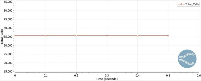
Mesh size of 0.0015m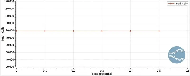

Comparison of supercycle intervals

Stage time interval	Temperature plot
0.01s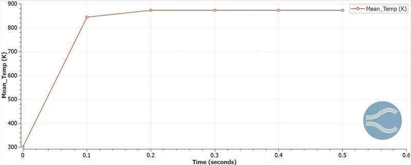
0.02s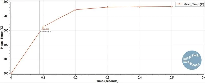
0.03s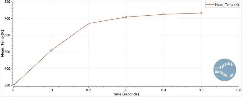

• The mass flow variation with time is shown above for different mesh size.
• Note that the inlet mass flow is negative,because the flow is entering the system.
• Whereas the outlet mass flow is positive,because the flow is leaving the system.
• The mass flow rate remains constant when the mesh size is varied, thus providing necessary proof for grid independency test.
• We can see from the above plots that the inlet pressure is higher than the outlet pressure due to the fact that heat addition to a flow causes the static and total pressure to drop at the outlet.
• The values of pressure remain constant and hence the grid independency is satisfied.
• The variation of flow velocity wth time is as shown in the figure above.
• Note that the inlet velocity is negative while the outlet flow velocity is positive
• The outlet flow velocity is higher in magnitude than the inlet velocity due to the fact that heat addition tp a subsonic flow results in flow acceleration
• The velocity values remain same irrespective of the mesh size thus proving the grid independency.
• Comparing the three mesh sizes, it is evident that the one with the smallest mesh size will obviously have the largest cell count and hence it will take more time to converge to the steady state answer.
• The total simulation time remains more or less the same, but the value of mean temperature varies as the stage interval is increased. Thus we get similar results for different values of stage interval in supercycling.

Thus the CHT simulation through a pipe is simulated and the results are discussed.

Animations of velocity

Mesh size	Velocity
Mesh size of 0.004m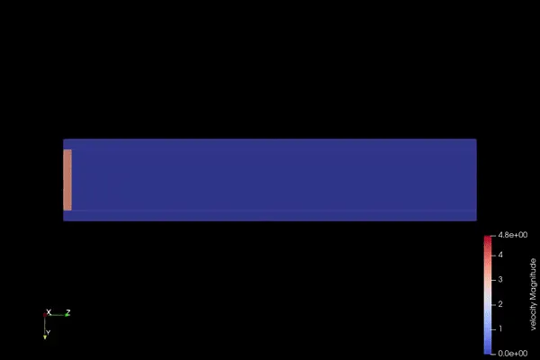
Mesh size of 0.002m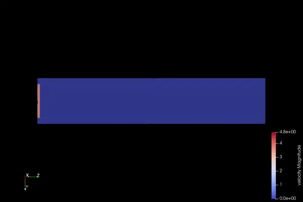
Mesh size of 0.0015m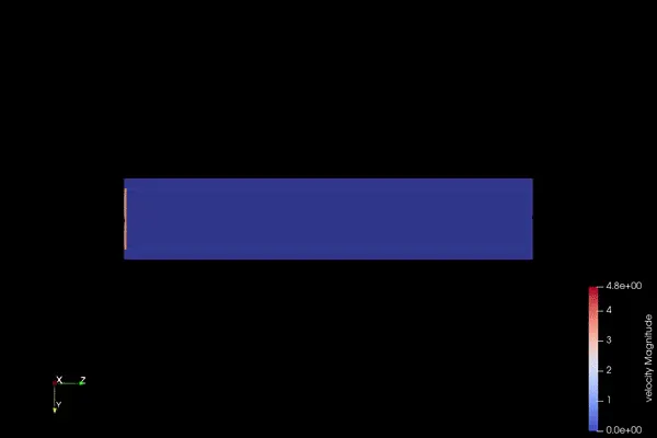