Week 12 - Validation studies of Symmetry BC vs Wedge BC in OpenFOAM vs Analytical H.P equation

AIM:

To continue the previous challenge by generalising the automation code for generating the blockmesh file for various angles(`theta=10^o ,25^o,45^o`) under various symmetry and wedge conditions subjected to initial velocity and pressure conditions

CONTINUATON:

A symmetric condition exists when a section of a pipe extends equally about an axis. A wedge condition is one in which the section is asymmetric about any given cross-sectional area.

To generate code for blockmeshdict file, a MATLAB code is written.

f1=fopen('blockMeshDict.txt','w');
l1='/*-----------------------------*- C++ -*---------------------------------*\';
l2='      =========                   |';
l3='      \\      /   F  ield         |  OpenFOAM: The Open Source CFD toolbox';
l4='       \\    /    O  peration     |  Website:  https://openfoam.org/';
l5='        \\  /     A  nd           |  Version:  9';
l6='         \\/      M  anipulation  |  ';
l7='\*-----------------------------------------------------------------------*/';
l8='FoamFile';
l9='{ ';
l10='    format    ascii;';
l11='    class     dictionary;';
l12='    object    blockMeshDict;';
l13='} ';
l14='// * * * * * * * * * * * * * * * * * * * * * * * * * * * * * * * * * * * *//';
l15='convertToMeters 1;';
l16=' ';
l17='vertices';
l18='(';
l19=');';
fprintf(f1,'%s\n',l1);
fprintf(f1,'%s\n',l2);
fprintf(f1,'%s\n',l3);
fprintf(f1,'%s\n',l4);
fprintf(f1,'%s\n',l5);
fprintf(f1,'%s\n',l6);
fprintf(f1,'%s\n',l7);
fprintf(f1,'%s\n',l8);
fprintf(f1,'%s\n',l9);
fprintf(f1,'%s\n',l10);
fprintf(f1,'%s\n',l11);
fprintf(f1,'%s\n',l12);
fprintf(f1,'%s\n',l13);
fprintf(f1,'%s\n',l14);
fprintf(f1,'%s\n',l15);
fprintf(f1,'%s\n',l16);
fprintf(f1,'%s\n',l17);
fprintf(f1,'%s\n',l18);
v=0.21;        %velocity of the flow
Re=2100;       %reynolds number of the flow
D=0.01;        %diameter in m
r=D/2;         %radius in m
L_h=0.06*Re*D; %entry length of the pipe
L=L_h+0.7;       %full length
v_max=2*v;     %max velocity
theta=input('Enter the value of the angle:');
%coordinates
c0=[0 0 0];    %zero coordinate
c1=[0 r*cosd(theta/2) r*sind(theta/2)];
c2=[0 r*cosd(theta/2) -r*sind(theta/2)];
c3=[L 0 0];
c4=[L r*cosd(theta/2) r*sind(theta/2)];
c5=[L r*cosd(theta/2) -r*sind(theta/2)];
d1=[300 50 1];  %number of divisions
gf=.2;            %grading factor
arc1=[0 r 0];    %arc passing through the point
arc2=[L r 0];    %arc passing through the point
fprintf(f1,'\t (%.3f %.6f %.3f) \n',c0);
fprintf(f1,'\t (%.3f %.6f %.7f) \n',c1);
fprintf(f1,'\t (%.3f %.6f %.7f) \n',c2);
fprintf(f1,'\t (%.3f %.6f %.3f) \n',c3);
fprintf(f1,'\t (%.3f %.6f %.7f) \n',c4);
fprintf(f1,'\t (%.3f %.3\3f %.7f) \n',c5);
fprintf(f1,'%s \n',l19);
fprintf(f1,'%s','blocks');
fprintf(f1,'\n%s','(');
fprintf(f1,'\t %s (%d %d %d) %s (1 %d 1)\n','hex (0 3 5 2 0 3 4 1)',d1,'simpleGrading',gf);
fprintf(f1,'\n%s',');');
fprintf(f1,'\n%s\n%s','edges','(');
fprintf(f1,'\n\t%s\t(%.3f %.3f %.3f)','arc 1 2',arc1);
fprintf(f1,'\n\t%s\t(%.3f %.3f %.3f)','arc 4 5',arc2);
fprintf(f1,'\n%s',');');
fprintf(f1,'\n%s\n%s','boundary','(');
fprintf(f1,'\n\t%s\n\t%s\n\t\t%s','inlet','{','type patch;');
fprintf(f1,'\n\t\t%s\n\t\t%s','faces','(');
fprintf(f1,'\n%25s\n\t\t%s\n\t%s','(0 1 2 0)',');','}');
fprintf(f1,'\n\t%s\n\t%s\n\t\t%s\n\t\t%s\n\t\t%s','outlet','{','type patch;','faces','(');
fprintf(f1,'\n%25s\n\t\t%s\n\t%s','(3 5 4 3)',');','}');
fprintf(f1,'\n\t%s\n\t%s\n\t\t%s\n\t\t%s\n\t\t%s','wall','{','type wall;','faces','(');
fprintf(f1,'\n%25s\n\t\t%s\n\t%s','(1 4 5 2)',');','}');
fprintf(f1,'\n\t%s\n\t%s\n\t\t%s\n\t\t%s\n\t\t%s','axis','{','type empty;','faces','(');
fprintf(f1,'\n%25s\n\t\t%s\n\t%s','(0 3 3 0)',');','}');
fprintf(f1,'\n\t%s\n\t%s\n\t\t%s\n%13s\n%9s','wedgeFront','{','type wedge;','faces','(');
fprintf(f1,'\n%25s\n\t\t%s\n\t%s','(0 3 4 1)',');','}');
fprintf(f1,'\n\t%s\n\t%s\n\t\t%s\n%13s\n%9s','wedgeBack','{','type wedge;','faces','(');
fprintf(f1,'\n%25s\n\t\t%s\n\t%s\n%s','(0 2 5 3)',');','}',');');
fprintf(f1,'\n%s\n%s\n%s','mergePatchPairs','(',');');

BLOCKMESH file:

/*-----------------------------*- C++ -*---------------------------------*\
      =========                   |
      \\      /   F  ield         |  OpenFOAM: The Open Source CFD toolbox
       \\    /    O  peration     |  Website:  https://openfoam.org/
        \\  /     A  nd           |  Version:  9
         \\/      M  anipulation  |  
\*-----------------------------------------------------------------------*/
FoamFile
{ 
    format    ascii;
    class     dictionary;
    object    blockMeshDict;
} 
// * * * * * * * * * * * * * * * * * * * * * * * * * * * * * * * * * * * *//
convertToMeters 1;
 
vertices
(
	 (0.000 0.000000 0.000) 
	 (0.000 0.004981 0.0004358) 
	 (0.000 0.004981 -0.0004358) 
	 (1.960 0.000000 0.000) 
	 (1.960 0.004981 0.0004358) 
	 (1.960 ); 
blocks
(	 hex (0 3 5 2 0 3 4 1) (300 50 1) simpleGrading (1 2.000000e-01 1)

);
edges
(
	arc 1 2	(0.000 0.005 0.000)
	arc 4 5	(1.960 0.005 0.000)
);
boundary
(
	inlet
	{
		type patch;
		faces
		(
                (0 1 2 0)
		);
	}
	outlet
	{
		type patch;
		faces
		(
                (3 5 4 3)
		);
	}
	wall
	{
		type wall;
		faces
		(
                (1 4 5 2)
		);
	}
	axis
	{
		type empty;
		faces
		(
                (0 3 3 0)
		);
	}
	wedgeFront
	{
		type wedge;
        faces
        (
                (0 3 4 1)
		);
	}
	wedgeBack
	{
		type wedge;
        faces
        (
                (0 2 5 3)
		);
	}
);
mergePatchPairs
(
);

A similar blockMeshDict file is generated for different angles.

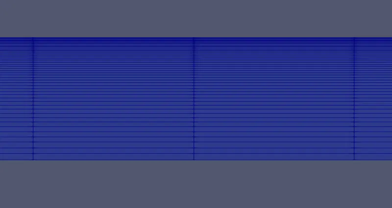
MESHING CONTOURS

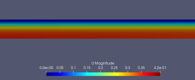
VELOCITY CONTOURS

POST-PROCESSING

To post-process data from excel file exported from openfoam into matlab, a code is also written.This stage involves comparing computational data with analytical data and drawing suitable inferences. For this case, the post processing is carried out in matlab. To do a comparison study between computational data and analytical data, we compare max velocity and shear stress values obtained in the calculation. A program is written in which the values(values of velocity and Pressure) that are obtained from Paraview are stored in an excel file and are read by matlab file.

data1=xlsread('All the files.xlsx','atx_1.3_10','A1:B1002');
data2=xlsread('All the files.xlsx','atx_1.3_25','A1:B1002');
data3=xlsread('All the files.xlsx','atx_1.3_45','A1:B1002');
data4=xlsread('All the files.xlsx','atx_1.3_10s','A1:B1002');
data5=xlsread('All the files.xlsx','atx_1.3_25s','A1:B1002');
data6=xlsread('All the files.xlsx','atx_1.3_45s','A1:B1002');
data7=xlsread('All the files.xlsx','over_length10','A1:C1002');
data8=xlsread('All the files.xlsx','over_length25','A1:C1002');
data9=xlsread('All the files.xlsx','over_length45','A1:C1002');
data10=xlsread('All the files.xlsx','over_length10s','A1:C1002');
data11=xlsread('All the files.xlsx','over_length25s','A1:C1002');
data12=xlsread('All the files.xlsx','over_length45s','A1:C1002');
point_for_all1=data1(:,1);
point_for_all2=data7(:,1);
vel_1=data1(:,2);
vel_2=data2(:,2);
vel_3=data3(:,2);
vel_4=data4(:,2);
vel_5=data5(:,2);
vel_6=data6(:,2);
vel_7=data7(:,2);
vel_8=data8(:,2);
vel_9=data9(:,2);
vel_10=data10(:,2);
vel_11=data11(:,2);
vel_12=data12(:,2);
pres_7=data7(:,3);
pres_8=data8(:,3);
pres_9=data9(:,3);
pres_10=data10(:,3);
pres_11=data11(:,3);
pres_12=data12(:,3);
%to calculate theoretical velocity distribution u=-(1/4mu)*(dp/dx)*(R^2-r^2)
mu=1e-03;
R=0.005;
r=linspace(0,0.005,1001);
dr=r(2)-r(1);
delp_dx=67.2;
vel_analyt=(1/(4*mu)).*(delp_dx).*(R^2-r.^2);
%to calculate analytical shear stress distribution
for i=2:length(vel_analyt)
    tau_analyt(i)=mu.*(vel_analyt(i)-vel_analyt(i-1))./dr;
end
%to calculate computed shear stress distribution
for i=2:length(vel_1)
    tau_computed(i)=mu.*(vel_1(i)-vel_1(i-1))./dr;
end
%to compare tau computed for different cases of wedge angle
%at theta=10
for i=2:length(vel_7)
    tau_10deg(i)=mu.*(vel_7(i)-vel_7(i-1))./dr;
end
%at theta=25
for i=2:length(vel_8)
    tau_25deg(i)=mu.*(vel_8(i)-vel_8(i-1))./dr;
end
%at theta=45
for i=2:length(vel_9)
    tau_45deg(i)=mu.*(vel_9(i)-vel_9(i-1))./dr;
end
%to compare tau computed for different cases of symmetry
%at theta=10
for i=2:length(vel_10)
    tau_10_s(i)=mu.*(vel_10(i)-vel_10(i-1))./dr;
end
%at theta=25
for i=2:length(vel_11)
    tau_25_s(i)=mu.*(vel_11(i)-vel_11(i-1))./dr;
end
%at theta=45
for i=2:length(vel_12)
    tau_45_s(i)=mu.*(vel_12(i)-vel_12(i-1))./dr;
end
%plotting all the values and comparing
%comparing velocity at distance 1.3m from entry of the pipe
figure(1)
plot(vel_1,point_for_all1,'r','linewidth',2);
hold on
plot(vel_2,point_for_all1,'b','linewidth',2);
hold on
plot(vel_3,point_for_all1,'g','linewidth',2);
hold on
plot(vel_4,point_for_all1,'c','linewidth',2);
hold on
plot(vel_5,point_for_all1,'m','linewidth',2);
hold on
plot(vel_6,point_for_all1,'y','linewidth',2);
hold off
xlabel('Velocity at distance of 1.3 m from entry');
ylabel('radial distance');
legend('velocity_{10 deg}','velocity_{25 deg}','velocity_{45 deg}',...
    'velocity_{10 symm}','velocity_{25 symm}','velocity_{45 symm}');
title('Velocity comparing symmetry and wedge boundary conditions');
hold off
%comparing velocity over the entire length of the pipe
figure(2)
plot(point_for_all2,vel_7,'r','linewidth',2);
hold on
plot(point_for_all2,vel_8,'b','linewidth',2);
hold on
plot(point_for_all2,vel_9,'g','linewidth',2);
hold on
plot(point_for_all2,vel_10,'c','linewidth',2);
hold on
plot(point_for_all2,vel_11,'m','linewidth',2);
hold on
plot(point_for_all2,vel_12,'y','linewidth',2);
xlabel('Length of the pipe');
ylabel('Velocity variation over the entire length of the pipe');
legend('velocity_{10 deg}','velocity_{25 deg}','velocity_{45 deg}',...
    'velocity_{10 symm}','velocity_{25 symm}','velocity_{45 symm}');
title('Velocity development along the length of the pipe for different angles');
hold off
%comparing pressure drop over the entire length of the pipe
figure(3)
plot(point_for_all2,pres_7,'r','linewidth',2);
hold on
plot(point_for_all2,pres_8,'b','linewidth',2);
hold on
plot(point_for_all2,pres_9,'g','linewidth',2);
hold on
plot(point_for_all2,pres_10,'c','linewidth',2);
hold on
plot(point_for_all2,pres_11,'m','linewidth',2);
hold on
plot(point_for_all2,pres_12,'y','linewidth',2);
xlabel('Length of the pipe');
ylabel('Pressure drop over the entire length of the pipe');
legend('Pressure_{10 deg}','Pressure_{25 deg}','Pressure_{45 deg}',...
    'Pressure_{10 symm}','Pressure_{25 symm}','Pressure_{45 symm}');
title('Pressure drop along the length of the pipe');
hold off

RESULTS AND DISCUSSIONS:

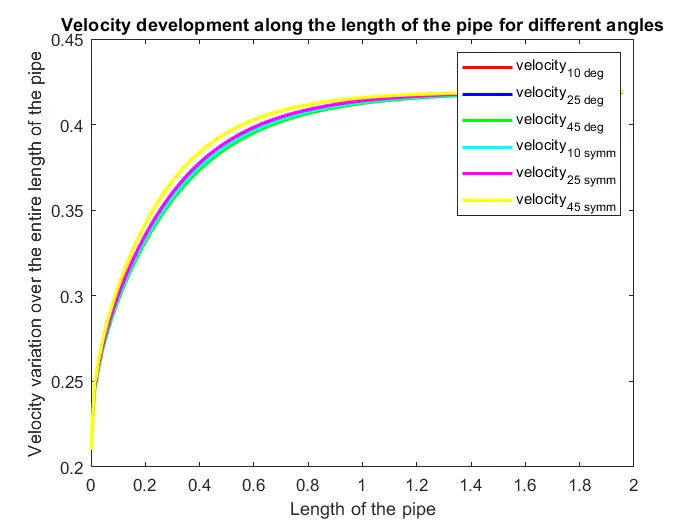
The plot shows variation of velocity over the entire length of the pipe. The variation between boundary conditions over symmetry and wedge boundary conditions is minimal, as is evident from the graph.

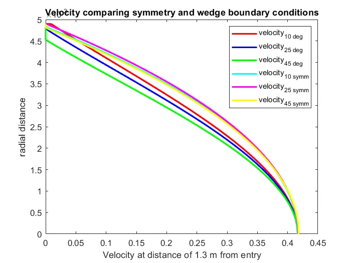
The plot shows variation of the velocity at a distance of x=1.3 m from the leading edge of the pipe. In this plot, we can observe that velocity variation for symmetry condition is very closer to the analytical variation.

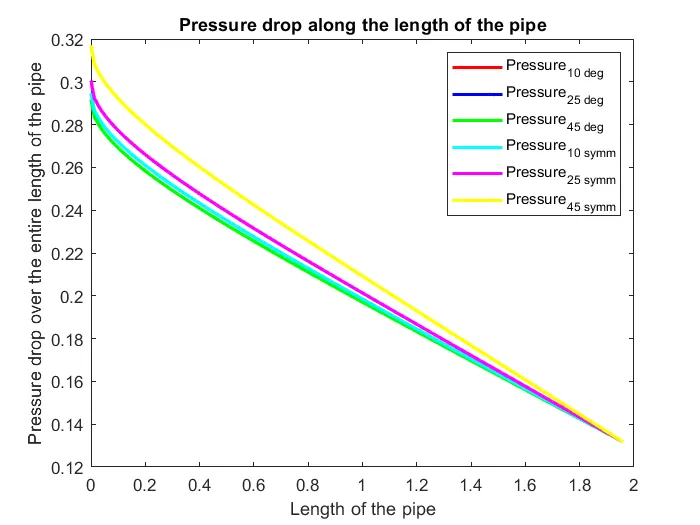
The plot shows variation of pressure along the length of the pipe. In this case, the case corresponding to 45degree symmetric boundary condition provides accurate results.

Thus, a comparison study is made between two types of boundary conditions. In some cases, a wedge condition is preferred because it offers a generalistic solution. A symmetry condition is used in axisymmetric flows. Comparing the above two sets of data given above, we can find that there is little to no variation of parameters between the two boundary conditions.