Week 4.1: Project - Steady state simulation of flow over a throttle body

Steady state simulation of flow in a throttle body

The aim of this challenge is to perform steady state simulation of flow over a throttle body and to

• Set up and run the steady state simulation for flow over throttle body.

• Post process the results and show pressure and velocity contours.

• Show the mesh (i.e surface with edges)

• Show the plots for pressure, velocity, mass flow rate and total cell count

Throttle Valve

A throttling valve can open, close and regulate media flow. Throttling valves are regulator valves. Some people use the term “control valves” to mean throttling valves. The truth is, there is a distinct line defining the two. Throttling valves have discs that do not only stop or start media flow. These discs can also regulate the amount, pressure and temperature of media passing through in any position prescribed.

Throttling valves will have a higher pressure at one end and a lower pressure at the other end. This closes the valve, depending on the degree of pressure. One such example is a diaphragm valve.

On the other hand, control valves will control the flow of media with the use of an actuator. It cannot function without one.

Pressure and temperature disrupt the flow of media so control valves regulate these. Also, these valves can change the flow or pressure conditions to match the required piping system conditions.

In this sense, control valves are specialized throttling valves. That being said, control valves can throttle but not all throttling valves are control valves.

The best example is the hydraulic system where an outside force has to release the vacuum so gas can enter the valve.

The Throttling Mechanism

When the pipeline use throttling valve, the media flow rate changes. When partially opening or closing the valve, there is a restriction in the flow of fluid. Thus, the control of media.

This, in turn, compacts the media in that partially opened valve. Molecules of the media begin to rub to each other. This creates friction. This friction additionally slows down media flow as it passes through the valve.

To better illustrate, think of the pipeline as the garden hose. Turning on, the water goes straight out the hose without any restriction. The flow is not strong. Now, think of the valve as the thumb partially covering the mouth of the hose.

The water that comes out changes in velocity and pressure because of the obstruction (the thumb). It is much stronger than the water that has not passed the valve yet. In the basic sense, this is throttling.

To apply this in the pipeline system, the system needs the cooler gas to be at the required hotter condition. With the throttling valve in place, gas temperature increases. This is due to molecules rubbing each other as they try to get out of the valve through a limited opening.

There is a broad range of uses for the throttling valves. Often one can find throttling valves in the following industrial applications:

● Air conditioning systems

● Refrigeration

● Hydraulics

● Steam applications

● High-temperature applications

● Pharmaceutical applications

● Chemical applications

● Food processing applications

● Fuel oil systems

Procedure

The procedure involves first setting up the model in Converge studio by marking boundaries and then setting up case in studio and then running the solution in cygwin and then postprocessing.

• At first, the model is imported.
• The geometry is then cleaned up by first finding fences and clicking on the outer surface and deleting it.
• The next step involves patching the inlet and outlet holes as shown below
• 
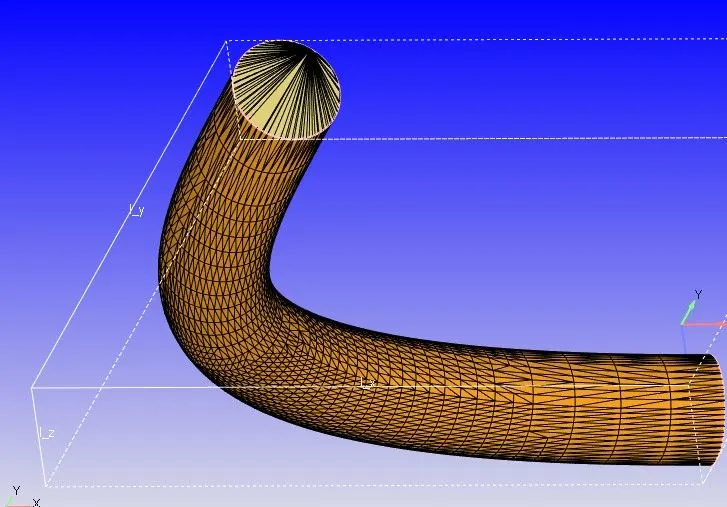
• Next step involves marking up boundaries. This is achieved as shown below:
• 
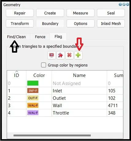
• Note that the four boundaries used are inlet, outlet, wall and throttle.
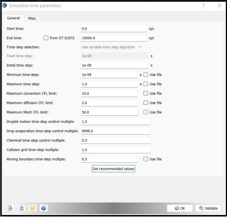
• Once the boundaries are marked, the next step is to setup simulation time parameters.
• Set the minimum timestep size as 1e-9(arbitrary) and fix the maximum timestep as 1.
• 
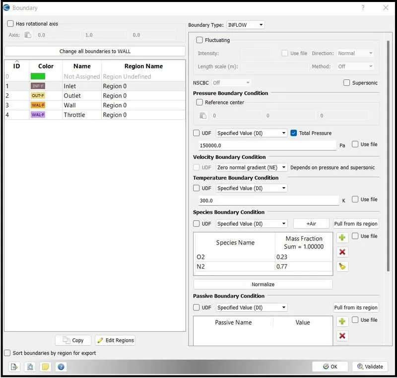
• Once done, next step is to setup boundary conditions.
• The inlet condition is marked as an inflow condition while the outlet condition is chosen as the outflow condition.
• The inlet pressure is given as 1.5e5 Pa whereas the outlet pressure is given as 1e5 Pa.
• The throttle and the wall boundaries are chosen as the wall boundary conditions.
• While considering rotation of throttle, the throttle boundary condition is chosen as rotating and the angle of rotation is specified.
• 
• Once provided, specify the basegrid mesh size appropriately(here, i used 0.002m).
• Once done, RNG turbulence model is chosen.
• To get better results at the throttle, an embedding is provided at the throttle valve as shown below:
• 
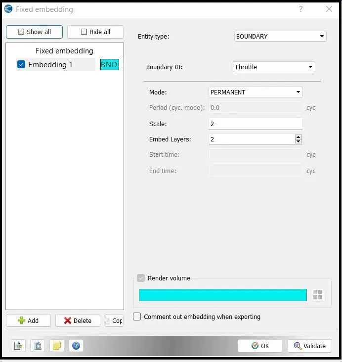
• The embed layer means that near the boundary specified(throttle), there will be two layers instead of one.
• Once done, export all the input files and save it in a file.
• Next step is to run the files in cygwin. Make sure to copy converge and mpi file to the destination folder.
• Open cygwin and go to the destination folder and type mpiexec.exe -n 2 converge.exe restricted
• The solver will run for a certain number of iterations.
• After which, postprocess the results in converge studio by choosing the file format to Paraview-VTK-inline format and convert them so that the results can be visualised in paraview.

Results and Discussions

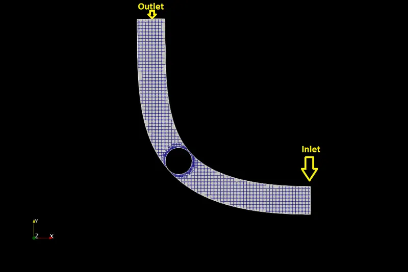
Size of mesh

The above mesh shows embedding closer to the throttle so as to get better flow visualizations. An embedding layer of 2 is provided which provides approximate results when the valve is set to motion. For better results, the mesh can be reduced a bit further depending upon the computer power. Note that the mesh near the wall are divided instead of a full mesh. Its due to adaptive meshing, which is a cool feature of converge studio.

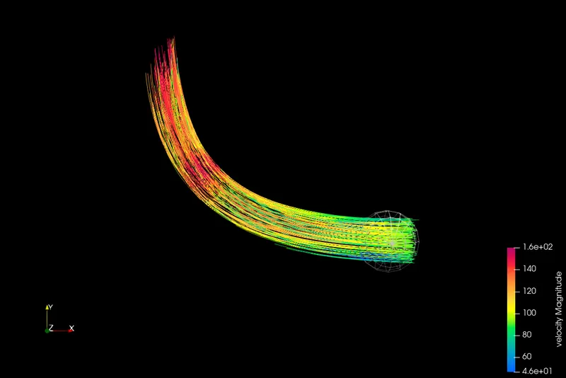
Streamlines of velocity

The above capture shows streamline plots of velocity. This is achieved by clicking on streamlines and choosing point source option and dragging the point at the inlet and click apply. Note that the streamlines at the inlet are in the velocity range of 60-80 m/s, but on reaching the throttle valve, the flow gets accelerated due to decrease in area which corresponds to an increment in velocity to satisfy massflow equation adn hence the velocity gets accelerated. We can provide no of seed points to see no.of streamlines that are actually visible.

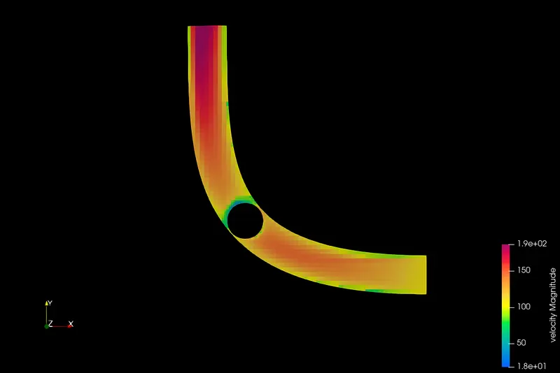
Contours of velocity

The above clip shows contours of velocity at a cross section(at the duct). Note that the velocity at the outlet is higher than that of the inlet. This is due to the conservation of continuity equation, which states for an incompressible flow(flow velocity is not as large to be considered compressible), decrease in area is accompanied by an increase in velocity. Note that the velocity drops to a very low value behind the valve due to flow separation phenomenon.

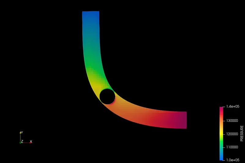
Contours of static pressure

The contours of static pressure shown above, also can be explained following similar explanation:Since there is a blockage, the pressure ahead of the throttle becomes higher, and this pressure is transmitted downstream as well as upstream to the flow thereby raising the pressure at the inlet. But once the flow crosses the throttle valve, it leaves behind a partial vacuum(flow separation region), thereby the pressure drops behind the throttle and the pressure at the outlet is lesser than the inlet.

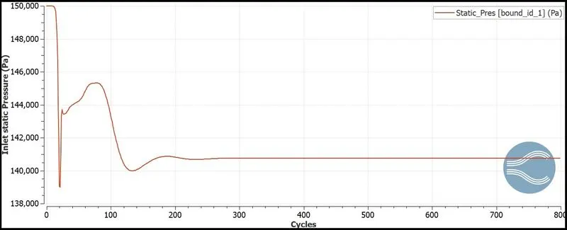
Chart of pressure variation over the no of cycles

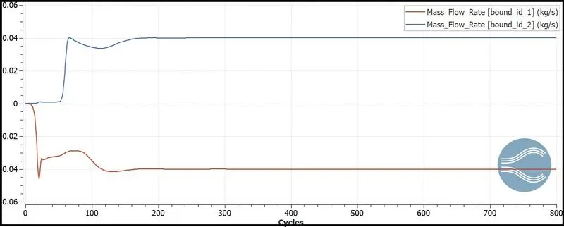
Chart of mass flow variation over the no of cycles

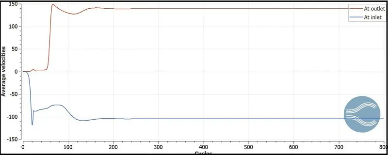
Chart of velocity variation over the no of cycles

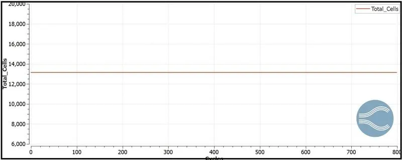
Count of total no of cells used here

The four plots shown above depict convergence of solution. Initially, we see a fluctuation of values, but after a certain number of cycles, the parameters attain steady state convergence. Note that the positive values of mass flow and velocity mean that the mass is leaving out of the system i.e. at the outlet, whereas a negative value of mass flow and velocity signify that the mass is entering the system i.e. at the inlet. It is also shown that the number of cell count is close to 12000, which is pretty good for a steady state approximation. Note that except for pressure, all other parameters achieve steady state close at 100 cycles but static pressure achieves steady state condition at 200 cycles.

Animation of pressure

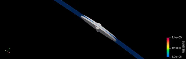The above shows an animation of static pressure variation when throttle angle is changed. Note that due to inclination, the static pressure increases more and more until the valve fully obstructs the flow, in which case there is a maximum buildup of pressure on the inlet side of the valve whereas the outlet side experiences a pressure considerably smaller than the inlet one.

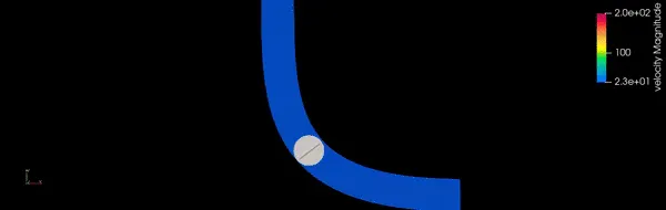
Animation of velocity

The velocity animation can be explained on a similar line as follows: because the area decreases more and more, the velocity increases proportionately until where no mass flows through to the other side of the valve and hence the velocity drops considerably at the outlet when the valve is fully closed.

Thus the steady state simulation through a throttle valve is simulated and the characteristics are studied and the animations and characteristic curves are shown.